When carrying out complex analysis, such as trend analysis, you may need to use a query as a DataSource. In these situations, rather than using transformation logic, try using Analysis Process Designer, which provides more flexibility and enables you to use queries as DataSources.
Key Concept
You can use Analysis Process Designer (APD) to run query result sets. In this scenario, APD serves as an extractor to load data in the background to a DataStore object (DSO) and then load master data to provide the query result data for analysis. This data is gathered from the query, stored in a direct-update DSO, and then passed to a master data InfoObject. You can use this technique to store snapshots of query result sets or to store the values of the query results.
Measures are often contained in queries that you need to extract for statistical analysis, trend analysis, or use in other queries for further analysis. If the data is strictly shown in queries, there is no standard DataSource that allows data loads directly from a query into a DataStore object (DSO) or InfoCube. Analysis Process Designer (APD) allows queries to run in the background. The resulting query data is extracted and stored for use in other queries.
This often-overlooked technique allows you to use query result data as a DataSource. You can use this technique to store trend analysis or extract complex result sets from a query that would be very difficult or impossible to do with transformation logic. This technique also provides the query designer the flexibility to create the various metrics needed for extraction.
For example, a company has a very complex measure called case fill rate, which is the number of cases shipped versus the number of cases ordered. This value is determined via some very involved logic using data from several InfoCubes and multifaceted query logic. The users want to store the case fill rate values each week and use the case fill rate as a factor to multiply by the weight of the shipments for each week. They want to store these values every week so that over time, past weeks can be analyzed and tracked for trends. This measure provides them with a good idea of what would have shipped. It allows the customer to get credit for product that the company could not fill by using the case fill rate as a factor for key figure values in the query.
In some circumstances, the query is the only source for a complex calculation. In models in which the queries are complex and data is determined from an aggregated value in the query process, the query is the only place to get these stored values. This is the case with this query. For the users to see their weekly case fill rate data from the query result set, it needs to be stored as master data to be used for future calculations. To provide this data, the only place the final case fill rate value is calculated is inside the case fill rate query. Duplicating the query logic into a transformation and loading data from the source into a case fill rate InfoCube is not possible because the level of granularity and the complex query logic does not allow this to be easily calculated using back-end transformation logic.
Data needs to be extracted each week by running the query, gathering the query results, and storing the result data historically. This data is constantly changing, so saving the weekly numbers provides a snapshot of the historical data values. It would be time consuming and cumbersome to run the report manually each week, record the result set, and store it somewhere in the SAP NetWeaver BW system. Therefore, to provide this data, I developed an automated APD process to mine the data from the query result sets and store the data by week.
In this process, data is extracted from a query and loaded into a DSO by ship-to and week. This data is then loaded into the master data so the case fill rate value can be used as an attribute in a formula variable in a query. APD extracts this data from the query, stores it in a DSO, loads it to a master data InfoObject, and finally uses the resulting case fill rate data in a query from the master data attributes. You can use this functionality and technique in SAP BW 3.x or SAP NetWeaver BW 7.0.
Note
The BI Expert knowledgebase has a number of articles about APD. For more information, go to Browse by Category >
Analysis Process Designer.
Analysis Process Designer
For this process I am using APD to run the case fill rate query in the background and store the query result sets by week in a DSO. To get started, I’ll walk through the APD setup.
A fill rate query is created with the necessary characteristics in the rows — in this case the week and the ship-to party. The query also has the Case Fill Rate Qty value in the query, along with other associated and relevant key figure values used to calculate the case fill rate (Figure 1). I have set up the query so that it only runs for the current week using a variable and determines the weekly case fill rate by ship-to party and week.

Figure 1
Case fill rate query reporting the week, ship-to party, case fill rate, and other key values
The APD process can load data into characteristic attributes of master data, DSOs, or flat files. There is no option to load data directly into InfoCubes or into key figure values stored as master data values. Because my goal is a master data table with the keys ship-to party and week along with the fill rate value as an attribute, I cannot enter the case fill rate key figure value directly into master data using the APD process. I can, however, load the data into a DSO first and then from the DSO data can be loaded into a master data InfoObject. This also allows me to have a DSO of this data in case I need it later for other types of reporting, while also providing a master data table with the case fill rate as an attribute for use in other queries.
Direct Update DSO
Data that is extracted using the APD to a DSO target can only be loaded to a special type of DSO called a direct update DSO. A direct update DSO differs from a traditional DSO in several ways. In a traditional DSO, data is stored in different versions (e.g., active, delta, modified), whereas a direct update DSO contains only an active version. Records with the same key are not aggregated, but simply overwritten and stored without SID generation for reporting in the same way the data comes from the source. Also, direct update DSOs are also not displayed in the administration or in the monitor. You do not see any loads when you manage the direct update DSO and view the requests tab after data is loaded.
You can set a DSO as a direct update when the DSO is created. A traditional DSO may also be switched to a direct update DSO as long as there is no data in the DSO (Figure 2). Use transaction RSA1, choose an InfoCube, right-click it, and then select the Edit InfoCubes option. In this screen you can see that this is a direct update DSO because the type in the Settings area of the DSO creation/change screen is set to Direct Update.

Figure 2
In the Settings area, you can see that the DSO is a Direct Update DSO
In my example, the key for the DSO is ship-to and week. This allows the case fill rate data to be stored with the granularity of week and ship-to. The case fill rate and related key figures from the query are also set up in the DSO. This allows each of these key figures to be populated in the DSO via the APD process. The query runs in the background and each of these key figure values is populated from the query based on the characteristics in the query source data.
APD Process
Now that you have a query defined and a corresponding direct-update DSO to house the data after the initial extraction, you are ready to setup the APD process. To start using APD, use transaction RSANWB (Figure 3).

Figure 3
Creation of the APD process using transaction RSANWB
The first step in creating the APD process is to establish the source of data. A DataSource for the APD process can be a file, master data attributes, a query, an InfoProvider, or a database table. In my example, the source of the data is the query I created in Figure 1. When the query icon is dragged into the work area, the system asks for the query that you want to use. You can then choose your fill rate query from the list of available queries (Figure 4). You have now specified the query that the system will use to run the APD process.
Tip!
When choosing queries that are good for the APD process, it is better to have smaller queries containing just the key figures and characteristics that are needed for the extraction. It is also important to make sure the variables are set to deliver a consistent dataset. This allows for a more efficient and better-performing extraction of data.

Figure 4
Query chosen as a DataSource from the APD process
Once the DataSource is chosen, the next step is to set the destination for the extracted data. This is called the data target in the APD process. In this example, the direct update DSO shown in Figure 2 is used to store the weekly case fill rate data. When the DSO icon from the Data Targets area is dragged into the work area, the system prompts for the DSO to be used as a target (Figure 5). Once the DSO is chosen, the next step to complete the APD process is to connect the query and the DSO for transformation.

Figure 5
Choose data target direct update DSO NAFL_O01 to store the data from the query
Transformation
The APD process transformation allows you to specify and map the fields in the APD DataSource and the fields in the APD data target. Not all fields in the DataSource or target are required to be mapped, but you need to map at least one field to allow for movement of data. In this case, the key figures in the query have a corresponding field in the DSO that mirrors that characteristic or key figure in length and type. The fields are mapped directly (Figure 6). Because all data in the query is already shown in cases, the case field is set to a constant unit of measure of CS (case).

Figure 6
APD transformation mapping of fields from the DataSource to the target DSO fields
Once the transformation is mapped from the DataSource to the data target, you can save and activate the APD. You can now run the activated APD process to gather the query result set for the current week into the DSO. Recall that once the process is completed, no requests are shown in the DSO when you manage the requests. You can view the data by looking at the contents of the direct update DSO, but you cannot see the requests in the monitor.
Click the execute icon to run the APD process in the background and move the data from the DataSource to the data target DSO. You can also schedule this process using a process chain to allow the system to perform the loads during the nightly batch loading process.
Master Data Case Fill Rate
After running the APD process, the data is stored for the current week in the direct update DSO. This DSO will house all historical fill rate data. To make the data available to the query and allow for its use in your calculations, you need to store the fill rate data into the master data with the compound key of week and ship-to. This master data allows the system to gather the data inside the query using the case fill rate key figure attribute of the master data and perform various calculations based on the fill rate via a formula variable.
To store this master data, you should create an InfoObject NASHIPFIL to store the data. NASHIPFIL should have the compound key of week and ship-to. The ship-to value is stored in NASHIPFIL and 0CALWEEK is set as a compound key (Figure 7).

Figure 7
NASHIPFIL master data InfoObject with the compound key of 0CALWEEK
The Fill Rate key figure, which is NAFILLRTE in my example, is set as a key figure attribute of the master data. This allows for the fill rate to be stored in the master data with the key ship-to and week, and later brought into a query via a formula variable (Figure 8).
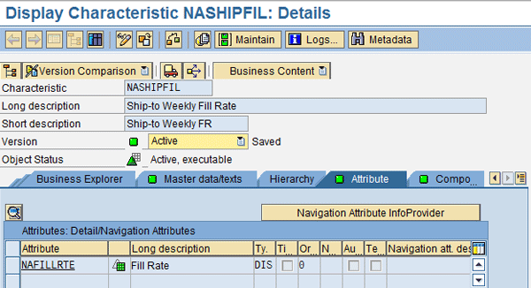
Figure 8
NASHIPFIL with the key figure attribute of Fill Rate
To load the data from the direct update DSO into the master data, you must build a transformation to move the corresponding data. The transformation maps from the ship-to to NASHIPFIL, week to 0CALWEEK, and the fill rate to the key figure NAFILLRTE (Figure 9). This allows the data to be extracted from the direct update DSO into the master data NASHIPFIL. I created a process chain to move the data from the direct update DSO into the master data NASHIPFIL. This process chain is scheduled to run in the weekly batch schedule.

Figure 9
Transformation mapping from the direct update DSO NAFL_O01 to NASHIPFIL master data
Using the Case Fill Rate in a Query
The last step in the process is to create a query that uses the case fill rate factor in a query. The goal is to multiply the case fill rate by the various shipped values in a corresponding week to determine the total shipped value if the realized fill rate is applied. Because the master data key is ship-to and week, you need to ensure that the InfoObjects 0CALWEEK (week) and NASHIPFIL (ship-to) are in the InfoProviders that are used for reporting. This enables a link to the key figure master data attribute NAFILLRTE (case fill rate) in the NASHIPFIL master data InfoObject. Therefore, each InfoCube already contains NASHIPFIL as a characteristic and the ship-to party is mapped to NASHIPFIL in the transformation.
0CALWEEK is also in each of the InfoCubes. It is mapped from 0CALDAY and contains the week and year of the transaction. This provides the link to the attribute of case fill rate NAFILLRTE from the master data NASHIPFIL. You then have weekly trending data by calendar week.
The query needs a formula variable with a replacement path to gather the case fill rate NAFILLRTE from the master data NASHIPFIL at runtime. This formula variable looks at the result set ship-to and week, looks up the corresponding fill rate from the master data, and applies that to the result set. To create a formula variable, use the formula variable option found when creating a formula and set the variable type as formula. Set the Processing By field to Replacement Path (Figure 10).
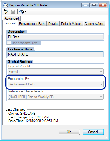
Figure 10
Formula variable using a replacement path
The Reference Characteristic from the formula variable in Figure 10 represents the key figure attribute that the formula variable returns. In my example, this is the NASHIPFIL (case fill rate) value. The system links to the NASHIPFIL master data table via the ship-to and week. The fill rate value for this attribute is filled in the Replacement Path tab in the formula value screen (Figure 11). By setting this option, the system populates the values into the variable. The fill rate attribute value is taken from the master data table and put into the query result set for use in the query calculation.
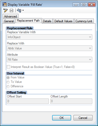
Figure 11
The Fill Rate attribute is populated into the Attribute field
APD Processing
You can use this APD process for loading data from a query any time you have data stored in query logic that is not easily reproduced during the load process. The data in the query can be run periodically and extracted into various data targets as a background process in batch.
This APD process can be used to load data for use as a multiplier in a query, as in this example, or the query result data can be stored as a snapshot of a specific time to serve as a base for trending reporting. For example, you could run a complex sales report to capture a snapshot of the values at the end of the month. These values could be stored in a DSO for trend analysis. This process works especially well in an environment where the past month’s data restate with each nightly load of master and transactional data. This gives you a true snapshot of the values at the end of the month, which allows you to trace trends from these values.