Shreekant Shiralkar and Rohit Kumar Das show how to apply SAP Predictive Analysis Library (PAL) functions in SAP HANA to retail store data to calculate an optimum price.
Key Concept
The Predictive Analysis Library (aka PAL) is a set of predictive algorithmic functions embedded in SAP HANA. Each of the algorithms is written in native C++ and is capable of execution at the database layer (i.e., in-memory computing). Execution at the database layer enables computing of an extremely large set of data with millions of rows in a few seconds. You can generate results in real time.
We demonstrate how PAL enables better business decision making with a case study that shows how to apply regression analysis over data clusters for a pricing strategy in the retail industry. You can predict the right price of an article at a future time, providing for higher profitability. Application of the k-means cluster analysis and multiple linear regression (MLR) algorithm is explained through step-by-step instructions. You can create relevant clusters and find relationships between different sales parameters in an electronic retail store to arrive at the optimized pricing for a product.
Note
This article is useful for SAP HANA developers and modelers who want to
develop predictive models using PAL as well as for data analysts who
want to identify the applicability of SAP HANA for predictive analytics.
Prerequisites
Following are the prerequisites for execution of PAL procedures in SAP HANA:
- The Application Function Library (AFL) is installed on SAP HANA. (Refer to section 4.1 and 4.2 of the SAP HANA Update and Configuration Guide available at https://www.saphana.com/docs/DOC-4048 or https://help.sap.com/hana/SAP_HANA_Update_and_Configuration_Guide_en.pdf.
- The AFL_WRAPPER_GENERATOR and AFL_WRAPPER_ERASER procedures should be created in the SYSTEM schema and you have EXECUTE privilege for these procedures.
- The AFL__SYS_AFL_AFLPAL_EXECUTE role is assigned to you.
- Transaction data sourced for running the algorithm does not contain any NULL value.
- Transaction data used does not have any duplicate entries.
- Basic knowledge of SAP HANA SQL scripting is required. (Refer to the SAP HANA SQL Script Reference available at https://help.sap.com/hana/SAP_HANA_SQL_Script_Reference_en.pdf).
- You have installed an SAP HANA client and SAP HANA studio in your desktop machine.
- To perform modeling activities you should have the following authorizations:
- SELECT privilege on _SYS_BI schema
- SELECT privilege in _SYS_BIC schema
- EXECUTE privilege on SYS.REPOSITORY_REST
- _SYS_BI_CP_ALL analytics privilege or any other relevant analytic privilege
- REPO.MAINTAIN_NATIVE_PACKAGE privilege on your system root package
In the following section we briefly cover various algorithms in PAL.
PAL Algorithms
- Association
- Clustering
- Classification
- Time series
- Preprocessing
- Statistics
- Social network analysis
- Miscellaneous
Table 1 shows the available algorithms and functions in the PAL as of SAP HANA Enterprise version 1.0 Support Package 8.
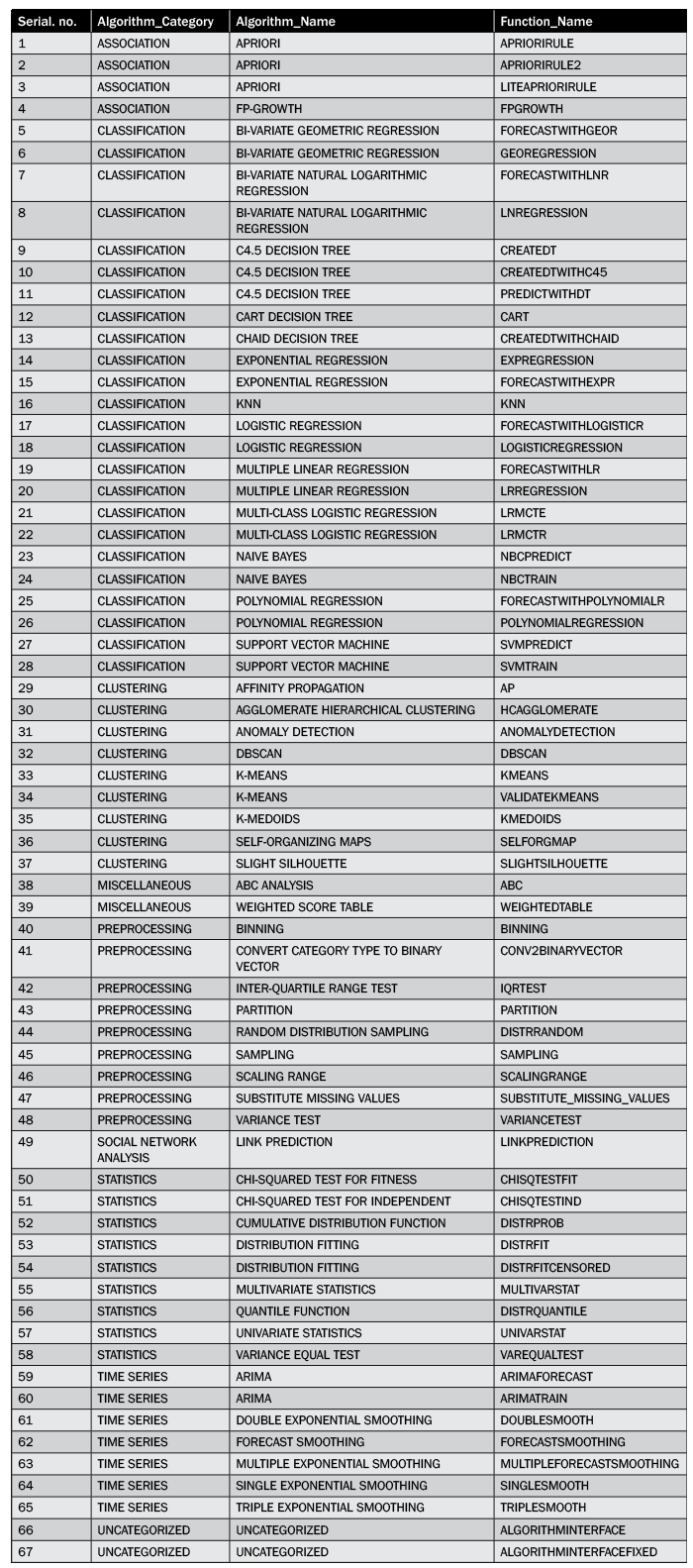
Table 1
Available SAP HANA PAL functions in SAP HANA Enterprise version 1.0 Support Package 8
Code to Check PAL Algorithms
To check the available PAL functions in your SAP HANA Enterprise installation, execute a SQL command in the SQL console of the SAP HANA Studio Modeler Perspective shown in Figure 1. You paste the SQL code provided in Figure 2 in the console. Then SQL is run using the execute icon to generate the output of the list of available PAL functions as shown in Figure 3.
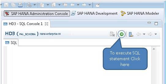
Figure 1
SAP HANA SQL Console
The SQL query shown in Figure 2 uses an AFL_FUNCTIONS database table that contains the information related to all the functions installed within the SAP HANA system. To learn how to access the SQL console, read the “Open SQL Console” section of step 2 in the “Step-By-Step Process” section.
SELECT

CASE

WHEN (FUNCTION_NAME in ('ANOMALYDETECTION','DBSCAN','KMEANS','VALIDATEKMEANS','SELFORGMAP','SLIGHTSILHOUETTE','HCAGGLOMERATE','AP','KMEDOIDS')) THEN 'CLUSTERING'

WHEN (FUNCTION_NAME in ('GEOREGRESSION','FORECASTWITHGEOR','LNREGRESSION','FORECASTWITHLNR','CREATEDT','PREDICTWITHDT','CREATEDTWITHCHAID','PREDICTWITHDT','EXPREGRESSION','FORECASTWITHEXPR','KNN','LOGISTICREGRESSION','FORECASTWITHLOGISTICR','LRREGRESSION','FORECASTWITHLR','NBCTRAIN','NBCPREDICT','POLYNOMIALREGRESSION','FORECASTWITHPOLYNOMIALR','SVMTRAIN','SVMPREDICT','CREATE_BINARY_TREE_MODEL','CREATEDTWITHC45','CART','LRMCTR','LRMCTE')) THEN 'CLASSIFICATION'

WHEN (FUNCTION_NAME in ('APRIORIRULE','LITEAPRIORIRULE','APRIORIRULE2','FPGROWTH')) THEN 'ASSOCIATION'

WHEN (FUNCTION_NAME in ('ARIMATRAIN','ARIMAFORECAST','SINGLESMOOTH','DOUBLESMOOTH','TRIPLESMOOTH','FORECASTSMOOTHING','MULTIPLEFORECASTSMOOTHING')) THEN 'TIME SERIES'

WHEN (FUNCTION_NAME in ('BINNING','CONV2BINARYVECTOR','IQRTEST','SAMPLING','SCALINGRANGE','VARIANCETEST','PARTITION','SUBSTITUTE_MISSING_VALUES','DISTRRANDOM')) THEN 'PREPROCESSING'

WHEN (FUNCTION_NAME in ('CHISQTESTFIT','UNIVARSTAT','MULTIVARSTAT','CHISQTESTIND','VAREQUALTEST','DISTRPROB','DISTRFIT','DISTRFITCENSORED','DISTRQUANTILE')) THEN 'STATISTICS'

WHEN (FUNCTION_NAME in ('LINKPREDICTION')) THEN 'SOCIAL NETWORK ANALYSIS'

WHEN (FUNCTION_NAME in ('ABC','WEIGHTEDTABLE')) THEN 'MISCELLANEOUS'

ELSE 'UNCATEGORIZED'

END as ALGORITHM_CATEGORY,

CASE

WHEN (FUNCTION_NAME IN ('AP')) THEN 'AFFINITY PROPAGATION'

WHEN (FUNCTION_NAME IN ('ANOMALYDETECTION')) THEN 'ANOMALY DETECTION '

WHEN (FUNCTION_NAME IN ('DBSCAN')) THEN 'DBSCAN '

WHEN (FUNCTION_NAME IN ('HCAGGLOMERATE')) THEN 'AGGLOMERATE HIERARCHICAL CLUSTERING '

WHEN (FUNCTION_NAME IN ('KMEANS','VALIDATEKMEANS')) THEN 'K-MEANS '

WHEN (FUNCTION_NAME IN ('SELFORGMAP')) THEN 'SELF-ORGANIZING MAPS '

WHEN (FUNCTION_NAME IN ('SLIGHTSILHOUETTE')) THEN 'SLIGHT SILHOUETTE '

WHEN (FUNCTION_NAME IN ('GEOREGRESSION','FORECASTWITHGEOR')) THEN 'BI-VARIATE GEOMETRIC REGRESSION '

WHEN (FUNCTION_NAME IN ('LNREGRESSION','FORECASTWITHLNR')) THEN 'BI-VARIATE NATURAL LOGARITHMIC REGRESSION '

WHEN (FUNCTION_NAME IN ('CREATEDT','PREDICTWITHDT','CREATEDTWITHC45','CREATE_BINARY_TREE_MODEL')) THEN 'C4.5 DECISION TREE '

WHEN (FUNCTION_NAME IN ('CREATEDTWITHCHAID','PREDICTWITHDT')) THEN 'CHAID DECISION TREE '

WHEN (FUNCTION_NAME IN ('EXPREGRESSION','FORECASTWITHEXPR')) THEN 'EXPONENTIAL REGRESSION '

WHEN (FUNCTION_NAME IN ('KNN')) THEN 'KNN '

WHEN (FUNCTION_NAME IN ('LOGISTICREGRESSION','FORECASTWITHLOGISTICR')) THEN 'LOGISTIC REGRESSION '

WHEN (FUNCTION_NAME IN ('LRREGRESSION','FORECASTWITHLR')) THEN 'MULTIPLE LINEAR REGRESSION '

WHEN (FUNCTION_NAME IN ('NBCTRAIN','NBCPREDICT')) THEN 'NAIVE BAYES '

WHEN (FUNCTION_NAME IN ('POLYNOMIALREGRESSION','FORECASTWITHPOLYNOMIALR')) THEN 'POLYNOMIAL REGRESSION '

WHEN (FUNCTION_NAME IN ('SVMTRAIN','SVMPREDICT')) THEN 'SUPPORT VECTOR MACHINE '

WHEN (FUNCTION_NAME IN ('APRIORIRULE','LITEAPRIORIRULE','APRIORIRULE2')) THEN 'APRIORI '

WHEN (FUNCTION_NAME IN ('SINGLESMOOTH')) THEN 'SINGLE EXPONENTIAL SMOOTHING '

WHEN (FUNCTION_NAME IN ('DOUBLESMOOTH')) THEN 'DOUBLE EXPONENTIAL SMOOTHING '

WHEN (FUNCTION_NAME IN ('TRIPLESMOOTH')) THEN 'TRIPLE EXPONENTIAL SMOOTHING '

WHEN (FUNCTION_NAME IN ('FORECASTSMOOTHING')) THEN 'FORECAST SMOOTHING '

WHEN (FUNCTION_NAME IN ('BINNING')) THEN 'BINNING '

WHEN (FUNCTION_NAME IN ('CONV2BINARYVECTOR')) THEN 'CONVERT CATEGORY TYPE TO BINARY VECTOR '

WHEN (FUNCTION_NAME IN ('IQRTEST')) THEN 'INTER-QUARTILE RANGE TEST '

WHEN (FUNCTION_NAME IN ('PARTITION')) THEN 'PARTITION '

WHEN (FUNCTION_NAME IN ('SAMPLING')) THEN 'SAMPLING '

WHEN (FUNCTION_NAME IN ('SCALINGRANGE')) THEN 'SCALING RANGE '

WHEN (FUNCTION_NAME IN ('SUBSTITUTE_MISSING_VALUES')) THEN 'SUBSTITUTE MISSING VALUES '

WHEN (FUNCTION_NAME IN ('VARIANCETEST')) THEN 'VARIANCE TEST '

WHEN (FUNCTION_NAME IN ('UNIVARSTAT')) THEN 'UNIVARIATE STATISTICS '

WHEN (FUNCTION_NAME IN ('MULTIVARSTAT')) THEN 'MULTIVARIATE STATISTICS '

WHEN (FUNCTION_NAME IN ('CHISQTESTFIT')) THEN 'CHI-SQUARED TEST FOR FITNESS '

WHEN (FUNCTION_NAME IN ('CHISQTESTIND')) THEN 'CHI-SQUARED TEST FOR INDEPENDENT '

WHEN (FUNCTION_NAME IN ('VAREQUALTEST')) THEN 'VARIANCE EQUAL TEST '

WHEN (FUNCTION_NAME IN ('LINKPREDICTION')) THEN 'LINK PREDICTION '

WHEN (FUNCTION_NAME IN ('ABC')) THEN 'ABC ANALYSIS '

WHEN (FUNCTION_NAME IN ('WEIGHTEDTABLE')) THEN 'WEIGHTED SCORE TABLE '

WHEN (FUNCTION_NAME IN ('MULTIPLEFORECASTSMOOTHING')) THEN 'MULTIPLE EXPONENTIAL SMOOTHING '

WHEN (FUNCTION_NAME IN ('ARIMATRAIN')) THEN 'ARIMA '

WHEN (FUNCTION_NAME IN ('ARIMAFORECAST')) THEN 'ARIMA '

WHEN (FUNCTION_NAME IN ('CART')) THEN 'CART Decision Tree '

WHEN (FUNCTION_NAME IN ('DISTRFIT')) THEN 'Distribution Fitting '

WHEN (FUNCTION_NAME IN ('DISTRFITCENSORED')) THEN 'Distribution Fitting '

WHEN (FUNCTION_NAME IN ('DISTRPROB')) THEN 'Cumulative Distribution Function '

WHEN (FUNCTION_NAME IN ('DISTRRANDOM')) THEN 'Random Distribution Sampling '

WHEN (FUNCTION_NAME IN ('DISTRQUANTILE')) THEN 'Quantile Function '

WHEN (FUNCTION_NAME IN ('FPGROWTH')) THEN 'FP-Growth '

WHEN (FUNCTION_NAME IN ('KMEDOIDS')) THEN 'K-Medoids '

WHEN (FUNCTION_NAME IN ('LRMCTR')) THEN 'Multi-Class Logistic Regression '

WHEN (FUNCTION_NAME IN ('LRMCTE')) THEN 'Multi-Class Logistic Regression '

ELSE 'UNCATEGORIZED'

END as ALGORITHM_NAME,

FUNCTION_NAME

FROM "SYS"."AFL_FUNCTIONS" WHERE AREA_NAME = 'AFLPAL' ORDER BY  1,2,3;CODE GOES HERE
Figure 2
SAP HANA SQL statement for finding available PAL functions in SAP HANA
Figure 3
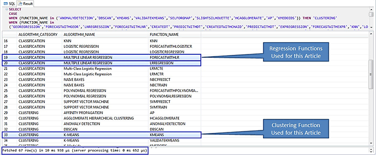
Figure 3
Screen output for available PAL functions
To find the optimum pricing strategy for the electronic store sales, k-means and MLR are the relevant algorithms. While k-means forms the cluster for similar products and price ranges, MLR helps find the pattern and relationship between the prices, products, regions, and discounts with the quantity sold within a period. With this analysis a company can decide on the best pricing or discounts for products for increasing sales. From the list of algorithms shown in Figure 3, we therefore focus on clustering using k-means and classification using the MLR algorithms.
Among the various algorithms available for cluster analysis, k-means is most widely used. It gives more accurate results than the others. K-means algorithm forms k number of clusters on the basis of various properties of the analysis object. Clustering helps to group objects with similar properties for further analysis. Classification is a process of identifying the data class for a set of data elements on the basis of their properties. The process of classifying the existing data elements is called training the model.
Once the data class has been identified, then new data elements can be classified using the training model thus formed. For example, for a sales scenario, sales revenues can be classified as poor, good, and excellent by considering products, margin, sales region, and month. After you complete this classification of sales revenues, you can predict the revenues for the upcoming months within any region and for any product. Figure 4 is an example of cluster analysis.
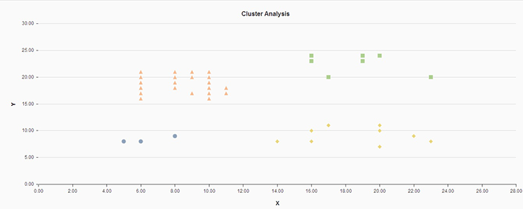
Figure 4
Cluster analysis
Linear regression is a statistical process for finding the relationships among variables—for example, product, price, region, discount quantity, and period. Figure 5 displays a simple example of regression analysis between region and month for sales revenue.
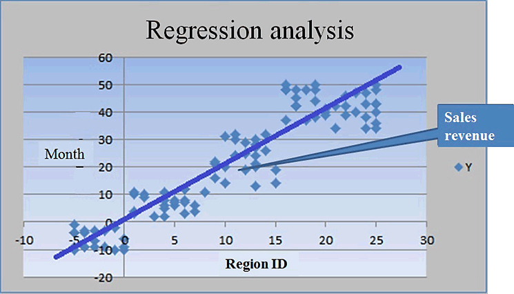
Figure 5
Classification or regression analysis
Business Scenario
This section explains the application of both cluster analysis and regression analysis to form relevant clusters and to find relationships between different sales parameters in an electronic retail store. The purpose is to find the optimal price for various products the store offers. Then we provide the step-by-step implementation procedure in SAP HANA.
Consider an electronic retail store that sells various electronic goods and accessories and provides various discounts on these products. The purchasing pattern for all these products depends on factors such as season, quarter, festival, and discounts. Because the store sells various products, clustering helps to form groups of similar products and ranges. Regression analysis helps to form relationships between the factors and determine (forecast) the correct price to gain maximum profitability.
Solution Overview
To decide on the pricing strategy for the electronic goods available within the store, we use predictive modeling. First, we group the data elements into clusters and then form the relationship between these data elements by performing the regression analysis.
Our business scenario includes PRODUCT, CITY, QUARTER, DISCOUNT, COST, and QUANTITY data elements for all the electronic goods sales available. We first group the data on the basis of product, city, quarter, discount, and cost, and form the cluster. Then we perform regression analysis on these data elements to find the relationship between product, city, quarter, discount, cost, and the quantity sold. Therefore, product, city, quarter, discount, and cost become the independent variables, and quantity depends on these independent variables.
To complete this procedure, follow these four steps:
- Log in to the SAP HANA system and prepare the system
- Create an input data table
- Create a wrapper procedure
- Create a calculation view
For this scenario we use the three PAL functions:
- Clustering: For our business scenario this algorithm uses electronic store data, which has three different categories of appliances, to partition data and forms clusters. For our case we use product, city, production cost, and discount percentage as the parameters on which to form the clusters.
- MLR: LRREGRESSION is the SAP HANA PAL function for MLR. By using the clusters thus formed by the k-means algorithm, LRREGRESSION forms the relationship between the quantity sold (dependent variable) to the product, city, production cost, and discount percentage.
- FORECASTWITHLR: FORECASTWITHLR is the SAP HANA PAL function for finding the expected values for the various object properties combination. After the relationship model is formed between the independent and dependent variables, FORECASTWITHLR accepts the dependent variable as input and predicts the quantity that is likely to be sold.
Step-by-Step Process
In the following sections we discuss the detailed steps for implementing the scenario using the PAL procedure and calculation view.
The steps we describe are executed in the modeler perspective of SAP HANA Studio. We explain the detailed steps to prepare data for procedure generation based on the three functions mentioned above. We also explain how to configure properties to match the price optimization use case. To create the types and database tables mentioned in the overview section, perform the following steps.
Step 1. Log in to SAP HANA Studio and Prepare the System
Open SAP HANA studio from your desktop machine. Go to Windows > Start > All Programs > SAP HANA > SAP HANA Studio as shown in Figure 6.
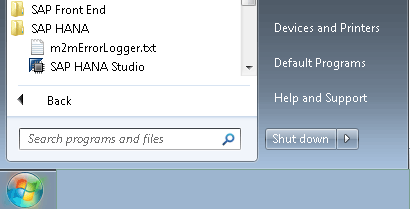
Figure 6
Launch SAP HANA studio
Open the Modeler perspective of SAP HANA studio by selecting Window > Open Perspective > Modeler from the menu bar. This action opens the screen shown in Figure 7. If the SAP HANA system is not already added, you need to add it to the SAP HANA studio. To do this, open the SAP HANA Systems view by selecting Window > Show View > SAP HANA Systems from the menu bar. Right-click the SAP HANA Systems view window on the left side of the screen and click the Add System... option as shown in Figure 7.
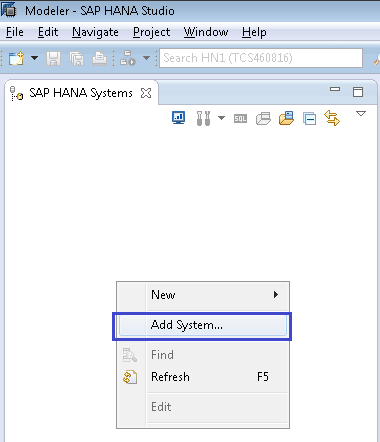
Figure 7
Add SAP HANA System - context menu selection
This action opens the screen shown in Figure 8. Populate the Host Name, Instance Number, and Description fields as shown in Figure 8. Leave the default settings for the other options. Click the Next button to proceed to the Connection Properties windows screen (Figure 9).
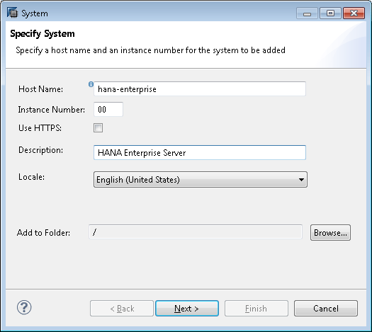
Figure 8
Add the SAP HANA system server details
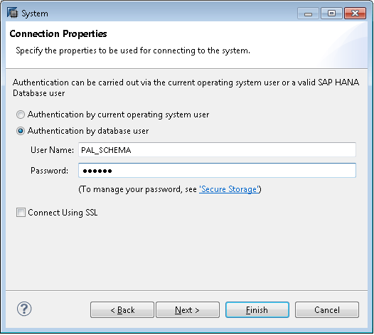
Figure 9
Add the SAP HANA system user name and password
In the Connection Properties screen, select the Authentication by database user button. Input the relevant data in the User Name and Password fields. Contact your SAP HANA administrator for the user ID and password for your SAP HANA server. Click the Next button to navigate to the Additional Properties screen (Figure 10).
Note
The host name entry is done in your client Microsoft Windows machine
from which you are accessing the SAP HANA server using SAP HANA studio.
The Hosts file is found in the OS Installed Drive:
WindowsSystem32driversetchosts file. To use a shortcut to open the
Hosts file and add an entry to it, log in to your Windows machine, go to
the Start menu, and open Run Command from the Accessories menu item.
The Run Command dialog appears on the screen. Input the text drivers
into the Run Command dialog and click the OK button. The drivers folder
window opens. Expand the etc folder within the drivers folder and open
the Hosts file within the etc folder with Notepad. Add the following
entry: <ip address>hana-enterprise. The <ip address> is the
IP address of the server where SAP HANA is installed. For your SAP HANA
server’s IP address, host name, and instance number, contact your SAP
HANA administrator.
In the Additional Properties screen (Figure 10) do not change any of the default selections. Click the Finish button. The system details and authentication information you provided are validated, and the system appears in the SAP HANA studio System view.

Figure 10
Add the SAP HANA system and review and finalize
Expand the system added from within the System view in SAP HANA studio. A folder tree structure consists of Catalog, Content, Provisioning, and Security folders. Expand the Catalog folder to check the catalog objects. The Catalog folder consists of schemas for which grants are provided to the schema user. In our example PAL_SCHEMA has access to the _SYS_AFL schema, which is required to run the PAL procedures.
Step 2. Create an Input Data Table
Create an Electronic DataStore table in the HANA PAL_SCHEMA schema using the SQL console.
Open SQL Console
Create the input data table structure using the SQL CREATE TABLE command in the SAP HANA SQL console. To open the SQL console, select the PAL_SCHEMA schema object and click the SQL console button as shown in Figure 11.

Figure 11
Launch the SQL console
A new SQL console window opens in SAP HANA studio as shown in Figure 12. When you open the SQL console with the PAL_SCHEMA user, it opens the console for the PAL_SCHEMA user. SYS_AFL is just a schema. By default the user schema is opened. If you want to change to SYS_AFL, you need to specifically run the command SET SCHEMA _SYS_AFL.
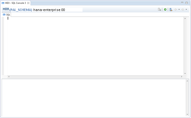
Figure 12
The SQL console view
Use the SQL code shown in Figure 13 to create the input database table definition in the PAL_SCHEMA schema. This table contains the structure of the input data table for the electronics store sales. This table is used for analyzing the clusters as well as the relationship among various columns.
-CREATE INPUT DATABASE TABLE

DROP TABLE "PAL_SCHEMA"."PR_OPT_ELECTRONIC_SALES";

CREATE COLUMN TABLE "PAL_SCHEMA"."PR_OPT_ELECTRONIC_SALES" (

            "AGGID" INTEGER,

            "PRODUCT_ID" INTEGER,

            "CITY_ID" INTEGER,

            "QUARTER_I" INTEGER,

            "YEAR" INTEGER,

            "QUANTITY" DOUBLE,

            "DISCOUNT_PER" DOUBLE,

            "SALES_REVENUE" DOUBLE,

            "UNIT_SELLING_PRICE" DOUBLE,

            "UNIT_PROD_COST" DOUBLE,

            "TOTAL_PROD_COST" DOUBLE,

            "PROFIT_PER" DOUBLE);
Figure 13
SQL statement to create an input database table
Figure 14 shows the input data that we use in our example.
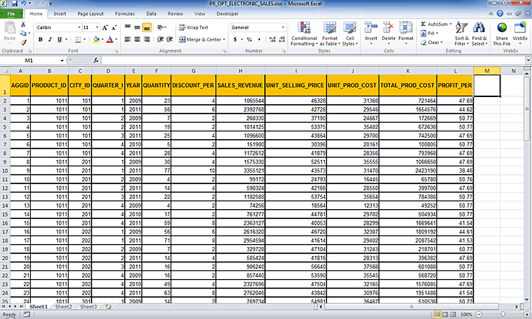
Figure 14
Input file (from a local PC)
To insert data into the table you created, create an Excel worksheet and import it using the SAP HANA import functionality. After you create the Excel sheet, complete these steps to import data. In SAP HANA studio, go to menu File > Import. Expand SAP HANA Content and choose Data from Local File as shown in Figure 15. Click the Next button to navigate to the Target System selection window as shown in Figure 16.

Figure 15
Data import: local file selection
Select the system from the list of systems shown in Figure 16. (In our example we added only one system, so there is only one item in the list.) Click the Next button to navigate to the Define Import Properties window shown in Figure 17.
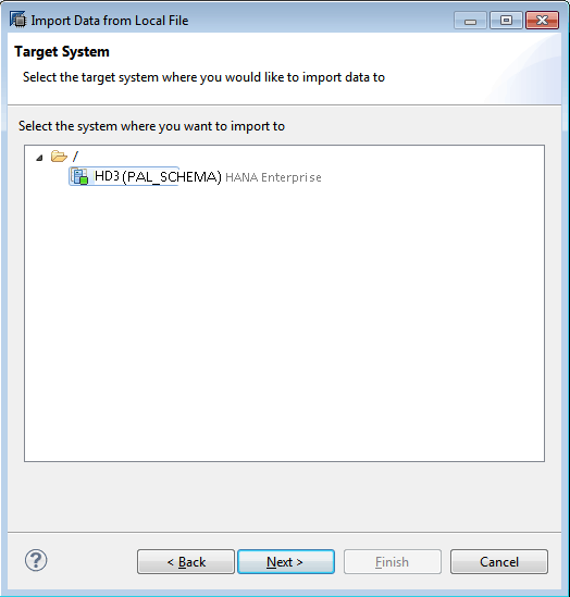
Figure 16
Data import: schema selection
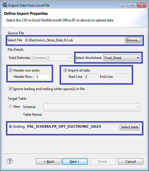
Figure 17
Data import: Excel file option selection
Select the source Excel file created using the Browse button. Choose the relevant worksheet from the Select Worksheet drop-down menu. Select the Header row exists check box if a header is available. Otherwise, leave it unchecked.
Select the Import all data check box. In the Target Table section select the Existing radio button to target the table already created and click the Select table button. A new table search window appears as shown in Figure 18.
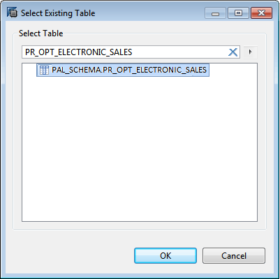
Figure 18
Search table
Type the name of the input table created in step 2 (Figure 13). Click the search icon  on the right. Search results are displayed in the same window with matching table names in the form of a list.
Select the relevant table name from the list and click the OK button to return to the Define Import Properties screen shown in Figure 17. Click the Next button to navigate to the Manage Table Definition and Data Mapping window shown in Figure 19.
Select the Map by Name option. Click the mapping menu icon  and then click the Finish button. That starts the process to load data into the table.
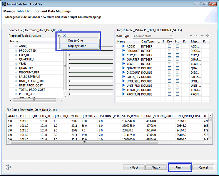
Figure 19
Data import: column mapping
After data is loaded into the table, you can view it using the Data Preview option. To view the table data, expand the Catalog folder within the System view of SAP HANA studio and expand the Tables folder to navigate to the Input table. Right-click the input table and select the Open Data Preview option from the context menu as shown in Figure 20.

Figure 20
Select the Open Data Preview option
A new tabbed window appears in which you can view data (Figure 21).

Figure 21
Data preview of the input table
Perform the below steps to create the PAL wrapper procedure. To make sure all objects are created within the user schema, set the schema to user schema by opening the SQL console. Input the following SQL statement: SET SCHEMA “PAL_SCHEMA”;.
Step 3. Create a Wrapper Procedure
To use all the PAL functions, you are required to create a wrapper procedure for the consumptions within one of the SAP HANA information views. The SYSTEM.AFL_WRAPPER_GENERATOR procedure takes this function as one of its input parameters and generates a wrapper PAL procedure for the data analysis. The AFL_WRAPPER_GENERATOR procedure requires four parameters to be passed:
- Procedure Name: This is the desired name of the PAL procedure to be created. This is user specified.
- Area Name: This is a constant value and should always be set to AFLPAL.
- Function Name: This is a PAL built-in function of the AFL library. For this use case it can be any of the three functions mentioned in the “Solution Overview” section.
- Signature Table: This is a user-defined table and contains records to describe the input table type, parameter table type, and result table type. Typically, a signature table is defined using a three-column table structure as shown in Table 2.
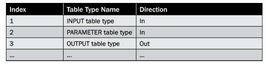
Table 2
Signature table template
PARAMETER values are different for various PAL functions. After you create all the types within the signature table, you can generate the PAL procedure by calling AFL_WRAPPER_GENERATOR using the command in Figure 22.
CALL SYSTEM.AFL_WRAPPER_GENERATOR('<procedure name>','AFLPAL',<PAL_FUNCTION>, <signature table>);
Figure 22
Generate wrapper procedure syntax
After you create the procedure, you can call it within the SQL console or in any other procedure using the command in Figure 23.
CALL <procedure name>(<input table>, <parameter table>, <result output table>, <PMML output table>) WITH overview;
Figure 23
Calling wrapper procedure syntax
Create K-Means Clustering Procedure
Clustering the electronic store sales data is required for our business scenario. To decide on the best pricing strategy, first data needs to be divided into meaningful clusters using the k-means algorithm. Using the concept provided in step 3, create the wrapper procedure for the k-means cluster algorithm to divide input data into clusters depending on the predefined criteria. Create table types for signature table parameters for k-means.
Create an input transaction table type using the command shown in Figure 24.
--CREATE INPUT DATA TYPE STRUCTURE FOR INPUT TO THE KMEANS AFL FUNCTION

DROP TYPE "PAL_SCHEMA"."TY_ELECTRONIC_SALES_KMEANS";

CREATE TYPE "PAL_SCHEMA"."TY_ELECTRONIC_SALES_KMEANS" AS TABLE (

            "AGGID" INTEGER,

            "PRODUCT_ID" INTEGER,

            "CITY_ID" INTEGER,

            "QUARTER_I" INTEGER,

            "DISCOUNT_PER" DOUBLE,

            "UNIT_PROD_COST" DOUBLE,

            "QUANTITY" DOUBLE

            );
Figure 24
Input table structure table type
Create an output result table type with the code in Figure 25.
--CREATE KMEANS RESULT TABLE TYPE STRUCTURE FOR OUTPUT TO KMEANS AFL FUNCTION
DROP TYPE "PAL_SCHEMA"."TY_KMEANS_RESULT";
CREATE TYPE "PAL_SCHEMA"."TY_KMEANS_RESULT" AS TABLE(
"AGGID" INTEGER,
"CLUSTER_NO" INTEGER,
"DISTANCE" DOUBLE
);
--CREATE KMEANS CENTER SUMMARY TABLE TYPE STRUCTURE FOR OUTPUT TO KMEANS AFL FUNCTION
DROP TYPE "PAL_SCHEMA"."TY_KMEANS_CENTERS";
CREATE TYPE "PAL_SCHEMA"."TY_KMEANS_CENTERS" AS TABLE(
"CENTER_CLID" INTEGER,
"PRODUCT_ID" INTEGER,
"CITY_ID" INTEGER,
"QUARTER_I" INTEGER,
"DISCOUNT_PER" DOUBLE,
"UNIT_PROD_COST" DOUBLE,
"QUANTITY" DOUBLE
);
Figure 25
K-means output table types
Create an input control table type using the code in Figure 26.
--CREATE INPUT PARAMA DATA TYPE STRUCTURE FOR INPUT TO THE KMEANS AFL FUNCTION
DROP TYPE "PAL_SCHEMA"."TY_PARAM_TABLE";
CREATE TYPE "PAL_SCHEMA"."TY_PARAM_TABLE" AS TABLE(
"PARAM_NAME" VARCHAR (50),
"INT_ARGS" INTEGER,
"DOUBLE_ARGS" DOUBLE,
"STRING_ARGS" VARCHAR (100));
Figure 26
Control table type for k-means
After you create the necessary table types, create the signature table, as described in step 3, and use the table types as input and output parameters, as shown in Table 3.
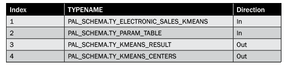
Table 3
Signature table for k-means
Create a signature table using the code shown in Figure 27.
C--CREATE INPUT PARAM TABLE FOR INPUT INTO THE AFL KMEANS FUNCTION "MAKE SURE THE COLUMN NAMES ARE EXACTLY THE SAME

-- ELSE ERROR WILL OCCUR

DROP TABLE "PAL_SCHEMA"."PR_OPT_IOPARAM";

CREATE COLUMN TABLE "PAL_SCHEMA"."PR_OPT_IOPARAM"( "ID" INTEGER, "TYPENAME" VARCHAR(50), "DIRECTION" VARCHAR(3));


INSERT INTO "PAL_SCHEMA"."PR_OPT_IOPARAM" VALUES (1, 'PAL_SCHEMA.TY_ELECTRONIC_SALES_KMEANS', 'in');

INSERT INTO "PAL_SCHEMA"."PR_OPT_IOPARAM" VALUES (2, 'PAL_SCHEMA.TY_PARAM_TABLE', 'in');

INSERT INTO "PAL_SCHEMA"."PR_OPT_IOPARAM" VALUES (3, 'PAL_SCHEMA.TY_KMEANS_RESULT', 'out');

INSERT INTO "PAL_SCHEMA"."PR_OPT_IOPARAM" VALUES (4, 'PAL_SCHEMA.TY_KMEANS_CENTERS', 'out');
Figure 27
Create a signature table for k-means
After you create all the necessary table types and signature table, create a wrapper procedure using the following steps:
1. Grant SELECT privilege on the signature table to the SYSTEM schema. Use the code in Figure 28.
GRANT SELECT ON "PAL_SCHEMA"."PR_OPT_IOPARAM" TO SYSTEM;
Figure 28
Grant SELECT privilege to the SYSTEM
Figure 29
--CREATE WRAPPER PROCEDURE FOR KMEANS

CALL "SYSTEM".AFL_WRAPPER_ERASER('PRC_ELEC_SALES_KMEANS');

CALL "SYSTEM".AFL_WRAPPER_GENERATOR('PRC_ELEC_SALES_KMEANS', 'AFLPAL', 'KMEANS', PR_OPT_IOPARAM);
Figure 29
CALL to AFL_PAL_WRAPPER functions to generate the wrapper procedure for k-means
Create the MLR Procedure
Our business scenario requires that we find out the quantity of a product that will be sold by changing the affecting parameters such as discounts. You use regression analysis to perform this relationship formation. To execute the regression analysis over the various clusters formed using the model created in the “Create K-Means Clustering Procedure” section, complete the following steps to create table types for signature table parameters for LRREGRESSION.
Create the input data table type using the command in Figure 30.
--CREATE INPUT DATA TYPE STRUCTURE FOR INPUT TO THE MLR AFL FUNCTION

DROP TYPE "PAL_SCHEMA"."TY_ELECTRONIC_SALES_MLR";

CREATE TYPE "PAL_SCHEMA"."TY_ELECTRONIC_SALES_MLR" AS TABLE (

            "AGGID" INTEGER,

            "QUANTITY" DOUBLE,                                         -- DEPENDANT VARIABLE

            "PRODUCT_ID" INTEGER,                                    -- INDEPENDANT VARIABLE

            "CITY_ID" INTEGER,                                              -- INDEPENDANT VARIABLE

            "QUARTER_I" INTEGER,                           -- INDEPENDANT VARIABLE

            "DISCOUNT_PER" DOUBLE,                                -- INDEPENDANT VARIABLE

            "UNIT_PROD_COST" DOUBLE                            -- INDEPENDANT VARIABLE

            );
Figure 30
Input data table type
Create the output result table type using the code in Figure 31.
--CREATE MLR RESULT TABLE TYPE STRUCTURE FOR OUTPUT TO MLR AFL FUNCTION

DROP TYPE "PAL_SCHEMA"."TY_MLR_RESULT";

CREATE TYPE "PAL_SCHEMA"."TY_MLR_RESULT" AS TABLE(

            "AGGID" INTEGER,

            "COEFICIENT" DOUBLE

            );


--CREATE MLR FITTED TABLE TYPE

DROP TYPE "PAL_SCHEMA"."TY_MLR_FITTED";

CREATE TYPE "PAL_SCHEMA"."TY_MLR_FITTED" AS TABLE(

            "AGGID" INTEGER,

            "FITTED" DOUBLE

            );


--CREATE MLR SIGNIFICANCE TABLE TYPE

DROP TYPE "PAL_SCHEMA"."TY_MLR_SIGNIFICANCE";

CREATE TYPE "PAL_SCHEMA"."TY_MLR_SIGNIFICANCE" AS TABLE(

            "NAME" VARCHAR,

            "VALUE" DOUBLE

            );


--CREATE MLR PMML MODEL TABLE TYPE

DROP TYPE "PAL_SCHEMA"."TY_MLR_PMML";

CREATE TYPE "PAL_SCHEMA"."TY_MLR_PMML" AS TABLE(

            "ID" INT,

            "MODEL" VARCHAR(5000)

            );
Figure 31
Output table types for regression
Use the input control table type already created in the “Create K-Means Clustering Procedure” section as an input parameter to the multiple linear regression signature table. Create the regression model. Reuse the signature database table PR_OPT_IOPARAM available in database schema PAL_SCHEMA and insert new values as shown in Table 4.
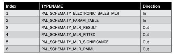
Table 4
Signature table for MLR
--USE ALREADY CREATED IOPARAM TABLE. INITIALIZE AND INSERT VALUES RELATED TO MLR FUNCTION

DELETE FROM "PAL_SCHEMA"."PR_OPT_IOPARAM";

INSERT INTO "PAL_SCHEMA"."PR_OPT_IOPARAM" VALUES (1,'PAL_SCHEMA.TY_ELECTRONIC_SALES_MLR','in');

INSERT INTO "PAL_SCHEMA"."PR_OPT_IOPARAM" VALUES (2,'PAL_SCHEMA.TY_PARAM_TABLE','in');

INSERT INTO "PAL_SCHEMA"."PR_OPT_IOPARAM" VALUES (3,'PAL_SCHEMA.TY_MLR_RESULT','out');

INSERT INTO "PAL_SCHEMA"."PR_OPT_IOPARAM" VALUES (4,'PAL_SCHEMA.TY_MLR_FITTED','out');

INSERT INTO "PAL_SCHEMA"."PR_OPT_IOPARAM" VALUES (5,'PAL_SCHEMA.TY_MLR_SIGNIFICANCE','out');

INSERT INTO "PAL_SCHEMA"."PR_OPT_IOPARAM" VALUES (6,'PAL_SCHEMA.TY_MLR_PMML','out');
Figure 32
Insert new values for MLR
Figure 33
--CREATE WRAPPER PROCEDURE FOR MLR

CALL "SYSTEM".AFL_WRAPPER_ERASER('PRC_ELEC_SALES_MLR');

CALL "SYSTEM".AFL_WRAPPER_GENERATOR('PRC_ELEC_SALES_MLR', 'AFLPAL', 'LRREGRESSION', PR_OPT_IOPARAM);
Figure 33
Generate a wrapper procedure for the MLR model
Create a Forecast with a Forecast MLR Procedure
After you create a clustering and regression model, use the forecast MLR (FMLR) function to use the trained model and forecast the values. To generate the FMLR model, complete the following steps. First, create table types for signature table parameters for FORECASTWITHLR to generate the predictive model.
Create the input data table type using the code in Figure 34.
--CREATE INPUT DATA TYPE STRUCTURE FOR INPUT TO THE FMLR AFL FUNCTION

DROP TYPE "PAL_SCHEMA"."TY_ELECTRONIC_SALES_FMLR";

CREATE TYPE "PAL_SCHEMA"."TY_ELECTRONIC_SALES_FMLR" AS TABLE (

            "AGGID" INTEGER,

            "PRODUCT_ID" INTEGER,                                    -- INDEPENDANT VARIABLE

            "CITY_ID" INTEGER,                                              -- INDEPENDANT VARIABLE

            "QUARTER_I" INTEGER,                           -- INDEPENDANT VARIABLE

            "DISCOUNT_PER" DOUBLE,                                -- INDEPENDANT VARIABLE

            "UNIT_PROD_COST" DOUBLE                            -- INDEPENDANT VARIABLE

            );
Figure 34
Input data table type for FMLR
Reuse output table type PAL_SCHEMA.TY_MLR_FITTED that you created earlier as output parameters within the signature table. The input control table type is reused as an input parameter within the signature table. Use the existing signature table (PR_OPT_IOPARAM of schema PAL_SCHEMA) and insert new values as shown in Table 5–for example, PAL_SCHEMA.TY_ELECTRONIC_SALES_FML.
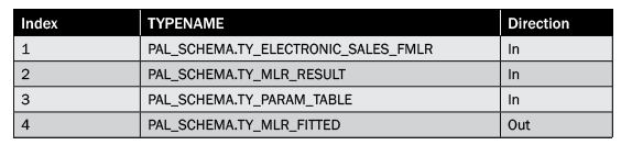
Table 5
Signature table for FMLR
When you specify the table names in SAP HANA, it uses the convention schema_name.table_name. The names within the SQL console are specified within the quotation marks to maintain the naming convention.
Insert new values into the control table using the code in Figure 35.
--USE ALREADY CREATED IOPARAM TABLE. INITIALIZE AND INSERT VALUES RELATED TO FMLR FUNCTION

DELETE FROM "PAL_SCHEMA"."PR_OPT_IOPARAM";

INSERT INTO "PAL_SCHEMA"."PR_OPT_IOPARAM" VALUES (1,'PAL_SCHEMA.TY_ELECTRONIC_SALES_FMLR','in');

INSERT INTO "PAL_SCHEMA"."PR_OPT_IOPARAM" VALUES (2,'PAL_SCHEMA.TY_MLR_RESULT','in');

INSERT INTO "PAL_SCHEMA"."PR_OPT_IOPARAM" VALUES (3,'PAL_SCHEMA.TY_PARAM_TABLE','in');

INSERT INTO "PAL_SCHEMA"."PR_OPT_IOPARAM" VALUES (4,'PAL_SCHEMA.TY_MLR_FITTED','out');
Figure 35
Insert into the control table for the FMLR
Generate the PAL wrapper procedure using the command in Figure 36.
-CREATE WRAPPER PROCEDURE FOR FMLR

CALL "SYSTEM".AFL_WRAPPER_ERASER('PRC_ELEC_SALES_FMLR');

CALL "SYSTEM".AFL_WRAPPER_GENERATOR('PRC_ELEC_SALES_FMLR', 'AFLPAL', 'FORECASTWITHLR', PR_OPT_IOPARAM);
Figure 36
Wrapper procedure generation for the FMLR
Create a Control Table
Create a common control parameter table for the three functions described in the previous sections with an ID and algorithm name for identifying the function. Use the code in Figure 37.
--CREATE CONTROL PARAMETER TABLE COMMON FOR ALL THE FUNCTIONS AND PROVIDE ID AND ALGORITHM NAME FOR IDENTIFYING THE FUNCTION

DROP TABLE "PAL_SCHEMA"."PR_OPT_PARAM_TABLE";

CREATE COLUMN TABLE "PAL_SCHEMA"."PR_OPT_PARAM_TABLE"(

            "ID" INTEGER,

            "ALGO_NAME" VARCHAR(5),

            "PARAM_NAME" VARCHAR (50),

            "INT_ARGS" INTEGER,

            "DOUBLE_ARGS" DOUBLE,

            "STRING_ARGS" VARCHAR (100));

-----------------------------------------

--INSERT VALUES FOR KMEANS

INSERT INTO "PAL_SCHEMA"."PR_OPT_PARAM_TABLE" VALUES (1,'KMEAN','THREAD_NUMBER', 4, null, null);

INSERT INTO "PAL_SCHEMA"."PR_OPT_PARAM_TABLE" VALUES (1,'KMEAN','GROUP_NUMBER', 3, null, null);

INSERT INTO "PAL_SCHEMA"."PR_OPT_PARAM_TABLE" VALUES (1,'KMEAN','INIT_TYPE', 1, null, null);

INSERT INTO "PAL_SCHEMA"."PR_OPT_PARAM_TABLE" VALUES (1,'KMEAN','DISTANCE_LEVEL',2, null, null);

INSERT INTO "PAL_SCHEMA"."PR_OPT_PARAM_TABLE" VALUES (1,'KMEAN','MAX_ITERATION', 100, null, null);

INSERT INTO "PAL_SCHEMA"."PR_OPT_PARAM_TABLE" VALUES (1,'KMEAN','EXIT_THRESHOLD', null, 1.0E-6, null);


-----------------------------------------

--INSERT VALUES FOR MLR

INSERT INTO "PAL_SCHEMA"."PR_OPT_PARAM_TABLE" VALUES (2,'MLREG','THREAD_NUMBER',4,null,null);


-------------------------------------------

--INSERT VALUES FOR FMLR

INSERT INTO "PAL_SCHEMA"."PR_OPT_PARAM_TABLE" VALUES (3,'FMLRG','THREAD_NUMBER',4,null,null);
Figure 37
Control table values to generate a predictive model
Step 4. Create a Calculation View
To consume the models and to call the generated procedures, create the calculation view in SAP HANA studio. The calculation view generates predictive output for currently available data and refreshes the model for any added data. Depending on the requirement, you may create a procedure for offline model creation and consume only the generated output. (Offline output generation and consumption are not areas on which I focus in this article.) To create the calculation view, perform the following steps:
Open SAP HANA studio as described in step 1. In the added system expand the Content folder. Right-click the Package name and select New > Package… as shown in Figure 38. A sub-package is created for keeping your work separate from other developers in case the root package is shared.
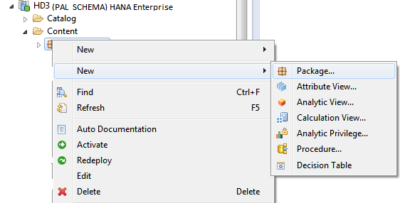
Figure 38
Create a package
Enter the sub-package Name and Description as shown in Figure 39. Click the OK button.
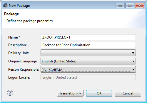
Figure 39
Define a package name
A new sub-package appears under the root package. Right-click the sub-package and select New > Calculation View… as shown in Figure 40.

Figure 40
Create a calculation view
This action opens the screen shown in Figure 41. In this screen enter the name of the calculation view in the Name field and a description in the Label field. In the Subtype field select SQL Script as shown in Figure 41. Click the Finish button to create a calculation view and open it in the SAP HANA studio workspace window.
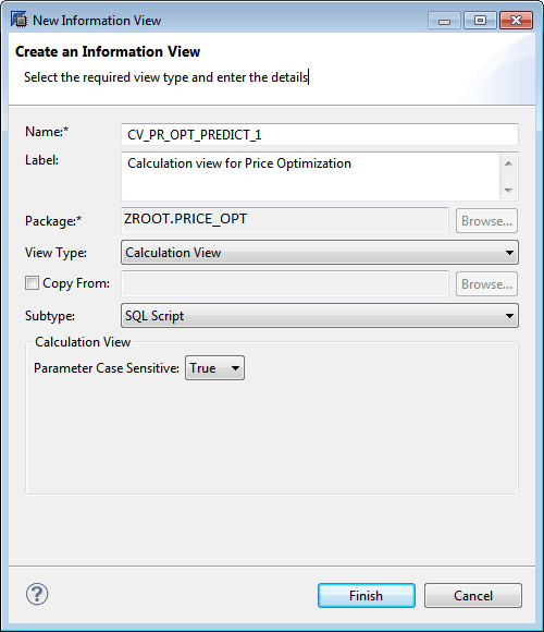
Figure 41
Set the calculation view property
The calculation view thus created has two nodes: Script_View and Semantics (Figure 42). The Script_View node is used to write the SAP HANA SQL script, and the Semantics node is used to define the properties of the output of the calculation view.
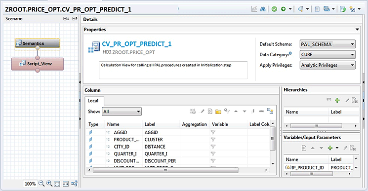
Figure 42
Calculation view scenario pane
When you click the Script_View node, the workspace view changes (Figure 43). Copy the SQL code shown in Figure 44 into the Details view, which is highlighted in Figure 43.
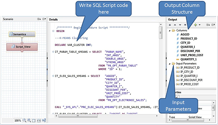
Figure 43
The Script view workspace
/********* Begin Procedure Script ************/
BEGIN
---K-MEANS Clustering
DECLARE VAR_CLUSTER INT;
IT_PARAM_TABLE_KMEANS = SELECT "PARAM_NAME",
"INT_ARGS",
"DOUBLE_ARGS",
"STRING_ARGS"
FROM "PR_OPT_PARAM_TABLE"
WHERE "ID" = 1;
IT_ELEX_SALES_KMEANS = SELECT "AGGID",
"PRODUCT_ID",
"CITY_ID",
"QUARTER_I",
"DISCOUNT_PER",
"UNIT_PROD_COST",
"QUANTITY"
FROM "PR_OPT_ELECTRONIC_SALES";
CALL "_SYS_AFL"."PRC_ELEC_SALES_KMEANS"(:IT_ELEX_SALES_KMEANS, :IT_PARAM_TABLE_KMEANS, IT_KMEANS_RESULT, IT_KMEANS_CENTERS) WITH OVERVIEW;
IT_ELEX_SALES_CLUSTER = SELECT A. "AGGID" AS "AGGID",
A."PRODUCT_ID" AS "PRODUCT_ID",
A."CITY_ID" AS "CITY_ID",
A."QUARTER_I" AS "QUARTER_I",
A."DISCOUNT_PER" AS "DISCOUNT_PER",
A."UNIT_PROD_COST" AS "UNIT_PROD_COST",
A."QUANTITY" AS "QUANTITY",
B."CLUSTER_NO" AS "CLUSTER_NO"
FROM :IT_KMEANS_RESULT B,
:IT_ELEX_SALES_KMEANS A
WHERE A.AGGID = B.AGGID;
---Multiple Linear Regression
IT_PARAM_TABLE_MLR = SELECT "PARAM_NAME",
"INT_ARGS",
"DOUBLE_ARGS",
"STRING_ARGS"
FROM "PR_OPT_PARAM_TABLE"
WHERE "ID" = 2;
IT_PARAM_TABLE_FMLR = SELECT "PARAM_NAME",
"INT_ARGS",
"DOUBLE_ARGS",
"STRING_ARGS"
FROM "PR_OPT_PARAM_TABLE"
WHERE "ID" = 3;
SELECT TOP 1 "CLUSTER_NO" INTO VAR_CLUSTER
FROM :IT_ELEX_SALES_CLUSTER
WHERE "PRODUCT_ID" = :IP_PRODUCT_ID
AND "CITY_ID" = :IP_CITY_ID
AND "QUARTER_I" = :IP_QUARTER_I
AND "UNIT_PROD_COST" >= :IP_PROD_COST;
IT_ELEX_SALES_FMLR_INPUT = SELECT 1 AS "AGGID",
TO_INT(:IP_PRODUCT_ID) AS "PRODUCT_ID",
TO_INT(:IP_CITY_ID) AS "CITY_ID",
TO_INT(:IP_QUARTER_I) AS "QUARTER_I",
TO_DOUBLE(:IP_DISCOUNT_PER) AS "DISCOUNT_PER",
TO_DOUBLE(:IP_PROD_COST) AS "UNIT_PROD_COST"
FROM DUMMY;
IF (:VAR_CLUSTER = 0)
THEN
IT_ELEX_SALES_CLUSTER_TEMP_1 = SELECT "CLUSTER_NO",
"AGGID",
"QUANTITY",
"PRODUCT_ID",
"CITY_ID",
"QUARTER_I",
"DISCOUNT_PER",
"UNIT_PROD_COST",
ROW_NUMBER() OVER (PARTITION BY "CLUSTER_NO" ORDER BY "AGGID") AS "ROW_NUM"
FROM :IT_ELEX_SALES_CLUSTER
WHERE "CLUSTER_NO" = 0
ORDER BY "PRODUCT_ID",
"CITY_ID",
"QUARTER_I",
"DISCOUNT_PER",
"UNIT_PROD_COST",
"QUANTITY";
IT_ELEX_SALES_CLUSTER_1 = SELECT "ROW_NUM" AS "AGGID",
"QUANTITY",
"PRODUCT_ID",
"CITY_ID",
"QUARTER_I",
"DISCOUNT_PER",
"UNIT_PROD_COST"
FROM :IT_ELEX_SALES_CLUSTER_TEMP_1
ORDER BY 1;
CALL _SYS_AFL.PRC_ELEC_SALES_MLR(:IT_ELEX_SALES_CLUSTER_1, :IT_PARAM_TABLE_MLR, IT_MLR_RESULT_1, IT_MLR_FITTED_1, IT_MLR_SIGNIFICANCE_1, IT_MLR_PMML_1);
CALL _SYS_AFL.PRC_ELEC_SALES_FMLR(:IT_ELEX_SALES_FMLR_INPUT, :IT_MLR_RESULT_1, :IT_PARAM_TABLE_FMLR, IT_FMLR_FITTED);
ELSEIF (:VAR_CLUSTER = 1)
THEN
IT_ELEX_SALES_CLUSTER_TEMP_2 = SELECT "CLUSTER_NO",
"AGGID",
"QUANTITY",
"PRODUCT_ID",
"CITY_ID",
"QUARTER_I",
"DISCOUNT_PER",
"UNIT_PROD_COST",
ROW_NUMBER() OVER (PARTITION BY "CLUSTER_NO" ORDER BY "AGGID") AS "ROW_NUM"
FROM :IT_ELEX_SALES_CLUSTER
WHERE "CLUSTER_NO" = 1
ORDER BY "PRODUCT_ID",
"CITY_ID",
"QUARTER_I",
"DISCOUNT_PER",
"UNIT_PROD_COST",
"QUANTITY";
IT_ELEX_SALES_CLUSTER_2 = SELECT "ROW_NUM" AS "AGGID",
"QUANTITY",
"PRODUCT_ID",
"CITY_ID",
"QUARTER_I",
"DISCOUNT_PER",
"UNIT_PROD_COST"
FROM :IT_ELEX_SALES_CLUSTER_TEMP_2
ORDER BY 1;
CALL _SYS_AFL.PRC_ELEC_SALES_MLR(:IT_ELEX_SALES_CLUSTER_2, :IT_PARAM_TABLE_MLR, IT_MLR_RESULT_2, IT_MLR_FITTED_2, IT_MLR_SIGNIFICANCE_2, IT_MLR_PMML_2);
CALL _SYS_AFL.PRC_ELEC_SALES_FMLR(:IT_ELEX_SALES_FMLR_INPUT, :IT_MLR_RESULT_2, :IT_PARAM_TABLE_FMLR, IT_FMLR_FITTED);
ELSE
IT_ELEX_SALES_CLUSTER_TEMP_3 = SELECT "CLUSTER_NO",
"AGGID",
"QUANTITY",
"PRODUCT_ID",
"CITY_ID",
"QUARTER_I",
"DISCOUNT_PER",
"UNIT_PROD_COST",
ROW_NUMBER() OVER (PARTITION BY "CLUSTER_NO" ORDER BY "AGGID") AS "ROW_NUM"
FROM :IT_ELEX_SALES_CLUSTER
WHERE "CLUSTER_NO" = 2
ORDER BY "PRODUCT_ID",
"CITY_ID",
"QUARTER_I",
"DISCOUNT_PER",
"UNIT_PROD_COST",
"QUANTITY";
IT_ELEX_SALES_CLUSTER_3 = SELECT "ROW_NUM" AS "AGGID",
"QUANTITY",
"PRODUCT_ID",
"CITY_ID",
"QUARTER_I",
"DISCOUNT_PER",
"UNIT_PROD_COST"
FROM :IT_ELEX_SALES_CLUSTER_TEMP_3
ORDER BY 1;
CALL _SYS_AFL.PRC_ELEC_SALES_MLR(:IT_ELEX_SALES_CLUSTER_3, :IT_PARAM_TABLE_MLR, IT_MLR_RESULT_3, IT_MLR_FITTED_3, IT_MLR_SIGNIFICANCE_3, IT_MLR_PMML_3);
CALL _SYS_AFL.PRC_ELEC_SALES_FMLR(:IT_ELEX_SALES_FMLR_INPUT, :IT_MLR_RESULT_3, :IT_PARAM_TABLE_FMLR, IT_FMLR_FITTED);
END IF;
-----FINAL output
IT_UNION_FMLR_FITTED = SELECT A."AGGID" AS "AGGID",
A."PRODUCT_ID" AS "PRODUCT_ID",
A."CITY_ID" AS "CITY_ID",
A."QUARTER_I" AS "QUARTER_I",
A."DISCOUNT_PER" AS "DISCOUNT_PER",
A."UNIT_PROD_COST" "UNIT_PROD_COST",
ROUND(ABS(B."FITTED"),0) AS "QUANTITY_1" FROM :IT_ELEX_SALES_FMLR_INPUT A,
:IT_FMLR_FITTED B
WHERE A.AGGID = B.AGGID;
var_out = SELECT * FROM :IT_UNION_FMLR_FITTED;
END /********* End Procedure Script ************/
Figure 44
SQL script code for the calculation view
Figure 43Figure 45
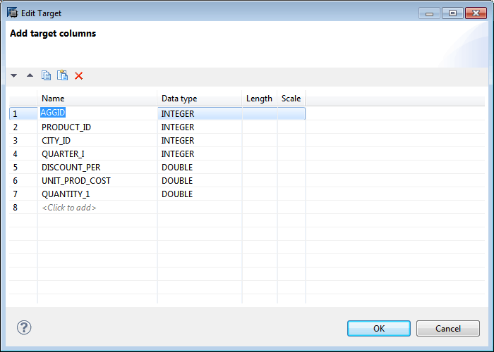
Figure 45
Create a calculation view target table
Create five input parameters within the calculation view — IP_PRODUCT_ID, IP_CITY_ID, IP_QUARTER_I, IP_DISCOUNT_PER, and IP_PROD_COST — for predicting the QUANTITY. The data type for input parameters is shown in Table 6. Calculation view input parameters can be created by right-clicking the Input Parameters folder in the Output pane as shown in Figure 43 and entering the names and data types for each parameter. Input parameters are used to take inputs from the users for forecasting.
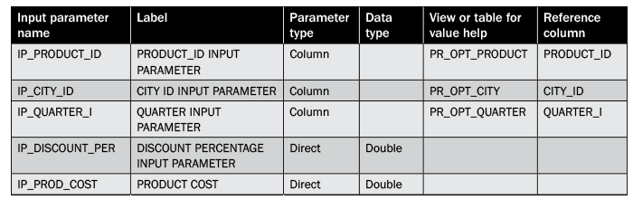
Table 6
Input parameter definitions
Figure 46 is a sample screen showing how to create IP_DISCOUNT_PER. Create other input parameters similarly. Enter data in the Name, Label, Parameter type, Data type View or table for value help and Reference column. Leave the default settings for the other fields, and click the OK button. The table for value help and the Reference column field are available only when the Parameter type is Column. These won’t appear for a direct parameter type.

Figure 46
Input parameter creation screen
In the Semantics view node of the calculation view, select Default Schema from the drop-down list in Properties as shown in Figure 42. In the Semantics view set the columns as Attributes or Measures depending on the column property. Define a type for each of the output columns as shown in Figure 47. Set all measurable columns as measures by clicking the type icon on the left of each of the column names and selecting a (aggregate function) measure from the dropdown in the cell on the right. The columns that provide input for the value of the measure are defined as attributes.
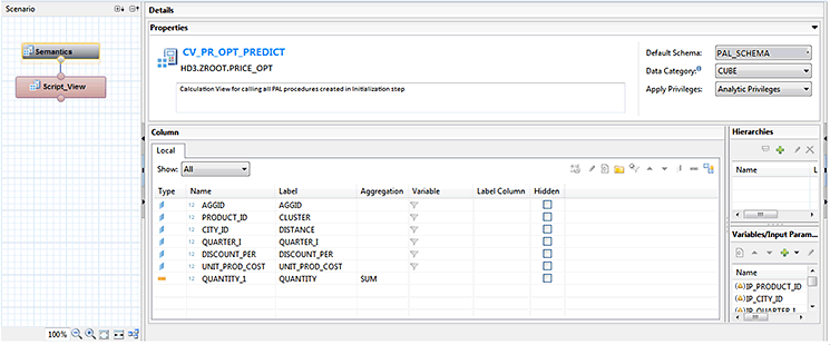
Figure 47
Set the columns as attributes or measures
Save and validate the view using the save and validate icon in Figure 48. After validation is successful, activate the calculation view using the activate icon. After successful activation of the calculation view, preview data using the data preview icon.

Figure 48
Validate and activate the calculation view, and then preview the data
After you click the data preview icon, the Variables and Input Parameters window appears (Figure 49). This screen displays the same input parameters that you created when creating the calculation view. Input the valid values for each parameter as shown in Figure 49 and click the OK button to visualize the results.
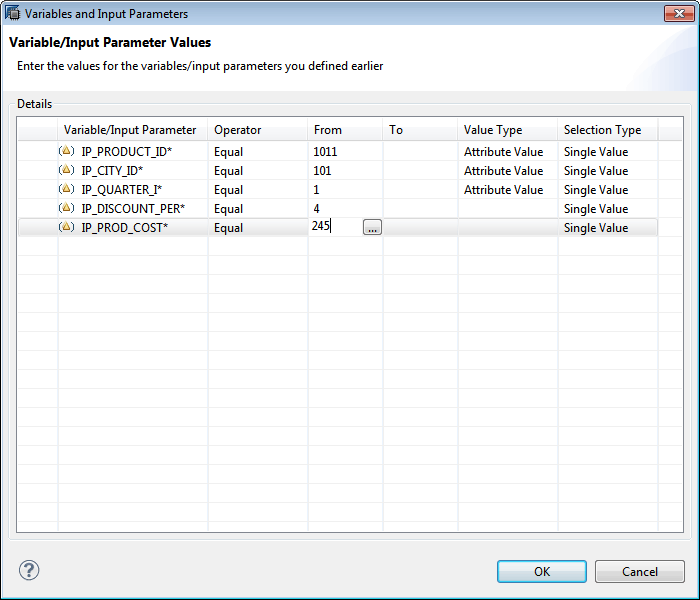
Figure 49
The Variable and Input Parameters screen
Click the Raw Data tab of the generated output window to see the quantity predicted as shown in Figure 50.
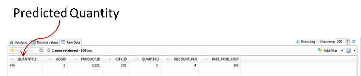
Figure 50
Output: the predicted quantity
You can create and execute a procedure based on a predictive algorithm. All the predictive algorithms follow the same generic procedure and can be implemented in similar fashion.
Figure 51 shows the complete SAP HANA SQL Script that combines all the steps that I explained for creating the Predictive Model. Figure 52 shows the SAP HANA SQL script for the calculation view to consume and apply the model on the input data.
--START OF PRICE OPTIMIZATION INITIALIZATION SCRIPT

SET SCHEMA PAL_SCHEMA;


-----INITIALIZATION FOR CLUSTERING (KMEANS) PAL ALGORITHM

--CREATE INPUT DATABASE TABLE

DROP TABLE "PAL_SCHEMA"."PR_OPT_ELECTRONIC_SALES";

CREATE COLUMN TABLE "PAL_SCHEMA"."PR_OPT_ELECTRONIC_SALES" (

            "AGGID" INTEGER,

            "PRODUCT_ID" INTEGER,

            "CITY_ID" INTEGER,

            "QUARTER_I" INTEGER,

            "YEAR" INTEGER,

            "QUANTITY" DOUBLE,

            "DISCOUNT_PER" DOUBLE,

            "SALES_REVENUE" DOUBLE,

            "UNIT_SELLING_PRICE" DOUBLE,

            "UNIT_PROD_COST" DOUBLE,

            "TOTAL_PROD_COST" DOUBLE,

            "PROFIT_PER" DOUBLE);

--CREATE EXCEL FILE FOR DATA INPUT AND IMPORT USING THE HANA IMPORT FUNCTIONALITY


--CREATE INPUT DATA TYPE STRUCTURE FOR INPUT TO THE KMEANS AFL FUNCTION

DROP TYPE "PAL_SCHEMA"."TY_ELECTRONIC_SALES_KMEANS";

CREATE TYPE "PAL_SCHEMA"."TY_ELECTRONIC_SALES_KMEANS" AS TABLE (

            "AGGID" INTEGER,

            "PRODUCT_ID" INTEGER,

            "CITY_ID" INTEGER,

            "QUARTER_I" INTEGER,

            "DISCOUNT_PER" DOUBLE,

            "UNIT_PROD_COST" DOUBLE,

            "QUANTITY" DOUBLE

            );


--CREATE KMEANS RESULT TABLE TYPE STRUCTURE FOR OUTPUT TO KMEANS AFL FUNCTION

DROP TYPE "PAL_SCHEMA"."TY_KMEANS_RESULT";

CREATE TYPE "PAL_SCHEMA"."TY_KMEANS_RESULT" AS TABLE(

            "AGGID" INTEGER,

            "CLUSTER_NO" INTEGER,

            "DISTANCE" DOUBLE

            );


--CREATE KMEANS CENTER SUMMARY TABLE TYPE STRUCTURE FOR OUTPUT TO KMEANS AFL FUNCTION

DROP TYPE "PAL_SCHEMA"."TY_KMEANS_CENTERS";

CREATE TYPE "PAL_SCHEMA"."TY_KMEANS_CENTERS" AS TABLE(

            "CENTER_CLID" INTEGER,

            "PRODUCT_ID" INTEGER,

            "CITY_ID" INTEGER,

            "QUARTER_I" INTEGER,

            "DISCOUNT_PER" DOUBLE,

            "UNIT_PROD_COST" DOUBLE,

            "QUANTITY" DOUBLE

            );


--CREATE INPUT PARAMA DATA TYPE STRUCTURE FOR INPUT TO THE KMEANS AFL FUNCTION

DROP TYPE "PAL_SCHEMA"."TY_PARAM_TABLE";

CREATE TYPE "PAL_SCHEMA"."TY_PARAM_TABLE" AS TABLE(

            "PARAM_NAME" VARCHAR (50),

            "INT_ARGS" INTEGER,

            "DOUBLE_ARGS" DOUBLE,

            "STRING_ARGS" VARCHAR (100));


--CREATE INPUT PARAM TABLE FOR INPUT INTO THE AFL KMEANS FUNCTION "MAKE SURE THE COLUMN NAMES ARE EXACTLY THE SAME

-- ELSE ERROR WILL OCCUR

DROP TABLE "PAL_SCHEMA"."PR_OPT_IOPARAM";

CREATE COLUMN TABLE "PAL_SCHEMA"."PR_OPT_IOPARAM"( "ID" INTEGER, "TYPENAME" VARCHAR(50), "DIRECTION" VARCHAR(3));


INSERT INTO "PAL_SCHEMA"."PR_OPT_IOPARAM" VALUES (1, 'PAL_SCHEMA.TY_ELECTRONIC_SALES_KMEANS', 'in');

INSERT INTO "PAL_SCHEMA"."PR_OPT_IOPARAM" VALUES (2, 'PAL_SCHEMA.TY_PARAM_TABLE', 'in');

INSERT INTO "PAL_SCHEMA"."PR_OPT_IOPARAM" VALUES (3, 'PAL_SCHEMA.TY_KMEANS_RESULT', 'out');

INSERT INTO "PAL_SCHEMA"."PR_OPT_IOPARAM" VALUES (4, 'PAL_SCHEMA.TY_KMEANS_CENTERS', 'out');


GRANT SELECT ON "PAL_SCHEMA"."PR_OPT_IOPARAM" TO SYSTEM;


--CREATE WRAPPER PROCEDURE FOR KMEANS

CALL "SYSTEM".AFL_WRAPPER_ERASER('PRC_ELEC_SALES_KMEANS');

CALL "SYSTEM".AFL_WRAPPER_GENERATOR('PRC_ELEC_SALES_KMEANS', 'AFLPAL', 'KMEANS', PR_OPT_IOPARAM);


-----INITIALIZATION FOR REGRESSION (MULTIPLE LINEAR REGRESSION) PAL ALGORITHM


--CREATE INPUT DATA TYPE STRUCTURE FOR INPUT TO THE MLR AFL FUNCTION

DROP TYPE "PAL_SCHEMA"."TY_ELECTRONIC_SALES_MLR";

CREATE TYPE "PAL_SCHEMA"."TY_ELECTRONIC_SALES_MLR" AS TABLE (

            "AGGID" INTEGER,

            "QUANTITY" DOUBLE,                                         -- DEPENDANT VARIABLE

            "PRODUCT_ID" INTEGER,                                   -- INDEPENDANT VARIABLE

            "CITY_ID" INTEGER,                                            -- INDEPENDANT VARIABLE

            "QUARTER_I" INTEGER,                         -- INDEPENDANT VARIABLE

            "DISCOUNT_PER" DOUBLE,                                -- INDEPENDANT VARIABLE

            "UNIT_PROD_COST" DOUBLE                            -- INDEPENDANT VARIABLE

            );


--CREATE MLR RESULT TABLE TYPE STRUCTURE FOR OUTPUT TO MLR AFL FUNCTION

DROP TYPE "PAL_SCHEMA"."TY_MLR_RESULT";

CREATE TYPE "PAL_SCHEMA"."TY_MLR_RESULT" AS TABLE(

            "AGGID" INTEGER,

            "COEFICIENT" DOUBLE

            );


--CREATE MLR FITTED TABLE TYPE

DROP TYPE "PAL_SCHEMA"."TY_MLR_FITTED";

CREATE TYPE "PAL_SCHEMA"."TY_MLR_FITTED" AS TABLE(

            "AGGID" INTEGER,

            "FITTED" DOUBLE

            );


--CREATE MLR SIGNIFICANCE TABLE TYPE

DROP TYPE "PAL_SCHEMA"."TY_MLR_SIGNIFICANCE";

CREATE TYPE "PAL_SCHEMA"."TY_MLR_SIGNIFICANCE" AS TABLE(

            "NAME" VARCHAR,

            "VALUE" DOUBLE

            );


--CREATE MLR PMML MODEL TABLE TYPE

DROP TYPE "PAL_SCHEMA"."TY_MLR_PMML";

CREATE TYPE "PAL_SCHEMA"."TY_MLR_PMML" AS TABLE(

            "ID" INT,

            "MODEL" VARCHAR(5000)

            );


--USE ALREADY CREATED IOPARAM TABLE. INITIALIZE AND INSERT VALUES RELATED TO MLR FUNCTION

DELETE FROM "PAL_SCHEMA"."PR_OPT_IOPARAM";

INSERT INTO "PAL_SCHEMA"."PR_OPT_IOPARAM" VALUES (1,'PAL_SCHEMA.TY_ELECTRONIC_SALES_MLR','in');

INSERT INTO "PAL_SCHEMA"."PR_OPT_IOPARAM" VALUES (2,'PAL_SCHEMA.TY_PARAM_TABLE','in');

INSERT INTO "PAL_SCHEMA"."PR_OPT_IOPARAM" VALUES (3,'PAL_SCHEMA.TY_MLR_RESULT','out');

INSERT INTO "PAL_SCHEMA"."PR_OPT_IOPARAM" VALUES (4,'PAL_SCHEMA.TY_MLR_FITTED','out');

INSERT INTO "PAL_SCHEMA"."PR_OPT_IOPARAM" VALUES (5,'PAL_SCHEMA.TY_MLR_SIGNIFICANCE','out');

INSERT INTO "PAL_SCHEMA"."PR_OPT_IOPARAM" VALUES (6,'PAL_SCHEMA.TY_MLR_PMML','out');


--CREATE WRAPPER PROCEDURE FOR MLR

CALL "SYSTEM".AFL_WRAPPER_ERASER('PRC_ELEC_SALES_MLR');

CALL "SYSTEM".AFL_WRAPPER_GENERATOR('PRC_ELEC_SALES_MLR', 'AFLPAL', 'LRREGRESSION', PR_OPT_IOPARAM);


------------------------


--CREATE INPUT DATA TYPE STRUCTURE FOR INPUT TO THE FMLR AFL FUNCTION

DROP TYPE "PAL_SCHEMA"."TY_ELECTRONIC_SALES_FMLR";

CREATE TYPE "PAL_SCHEMA"."TY_ELECTRONIC_SALES_FMLR" AS TABLE (

            "AGGID" INTEGER,

            "PRODUCT_ID" INTEGER,                                   -- INDEPENDANT VARIABLE

            "CITY_ID" INTEGER,                                            -- INDEPENDANT VARIABLE

            "QUARTER_I" INTEGER,                         -- INDEPENDANT VARIABLE

            "DISCOUNT_PER" DOUBLE,                                -- INDEPENDANT VARIABLE

            "UNIT_PROD_COST" DOUBLE                            -- INDEPENDANT VARIABLE

            );


--USE ALREADY CREATED IOPARAM TABLE. INITIALIZE AND INSERT VALUES RELATED TO FMLR FUNCTION

DELETE FROM "PAL_SCHEMA"."PR_OPT_IOPARAM";

INSERT INTO "PAL_SCHEMA"."PR_OPT_IOPARAM" VALUES (1,'PAL_SCHEMA.TY_ELECTRONIC_SALES_FMLR','in');

INSERT INTO "PAL_SCHEMA"."PR_OPT_IOPARAM" VALUES (2,'PAL_SCHEMA.TY_MLR_RESULT','in');

INSERT INTO "PAL_SCHEMA"."PR_OPT_IOPARAM" VALUES (3,'PAL_SCHEMA.TY_PARAM_TABLE','in');

INSERT INTO "PAL_SCHEMA"."PR_OPT_IOPARAM" VALUES (4,'PAL_SCHEMA.TY_MLR_FITTED','out');


--CREATE WRAPPER PROCEDURE FOR FMLR

CALL "SYSTEM".AFL_WRAPPER_ERASER('PRC_ELEC_SALES_FMLR');

CALL "SYSTEM".AFL_WRAPPER_GENERATOR('PRC_ELEC_SALES_FMLR', 'AFLPAL', 'FORECASTWITHLR', PR_OPT_IOPARAM);


--CREATE CONTROL PARAMETER TABLE COMMON FOR ALL THE FUNCTIONS AND PROVIDE ID AND ALGORITHM NAME FOR IDENTIFYING THE FUNCTION

DROP TABLE "PAL_SCHEMA"."PR_OPT_PARAM_TABLE";

CREATE COLUMN TABLE "PAL_SCHEMA"."PR_OPT_PARAM_TABLE"(

            "ID" INTEGER,

            "ALGO_NAME" VARCHAR(5),

            "PARAM_NAME" VARCHAR (50),

            "INT_ARGS" INTEGER,

            "DOUBLE_ARGS" DOUBLE,

            "STRING_ARGS" VARCHAR (100));

-----------------------------------------

--INSERT VALUES FOR KMEANS

INSERT INTO "PAL_SCHEMA"."PR_OPT_PARAM_TABLE" VALUES (1,'KMEAN','THREAD_NUMBER', 4, null, null);

INSERT INTO "PAL_SCHEMA"."PR_OPT_PARAM_TABLE" VALUES (1,'KMEAN','GROUP_NUMBER', 3, null, null);

INSERT INTO "PAL_SCHEMA"."PR_OPT_PARAM_TABLE" VALUES (1,'KMEAN','INIT_TYPE', 1, null, null);

INSERT INTO "PAL_SCHEMA"."PR_OPT_PARAM_TABLE" VALUES (1,'KMEAN','DISTANCE_LEVEL',2, null, null);

INSERT INTO "PAL_SCHEMA"."PR_OPT_PARAM_TABLE" VALUES (1,'KMEAN','MAX_ITERATION', 100, null, null);

INSERT INTO "PAL_SCHEMA"."PR_OPT_PARAM_TABLE" VALUES (1,'KMEAN','EXIT_THRESHOLD', null, 1.0E-6, null);


-----------------------------------------

--INSERT VALUES FOR MLR

INSERT INTO "PAL_SCHEMA"."PR_OPT_PARAM_TABLE" VALUES (2,'MLREG','THREAD_NUMBER',4,null,null);


-------------------------------------------

--INSERT VALUES FOR FMLR

INSERT INTO "PAL_SCHEMA"."PR_OPT_PARAM_TABLE" VALUES (3,'FMLRG','THREAD_NUMBER',4,null,null);


--END OF PRICE OPTIMIZATION INITIALIZATION SCRIPT
Figure 51
Complete SAP HANA procedure: initialization script
Figure 52 includes the script code for a complete procedure using a SAP HANA calculation view.
/********* Begin Procedure Script ************/
BEGIN
---K-MEANS Clustering
DECLARE VAR_CLUSTER INT;
IT_PARAM_TABLE_KMEANS = SELECT "PARAM_NAME",
"INT_ARGS",
"DOUBLE_ARGS",
"STRING_ARGS"
FROM "PR_OPT_PARAM_TABLE"
WHERE "ID" = 1;
IT_ELEX_SALES_KMEANS = SELECT "AGGID",
"PRODUCT_ID",
"CITY_ID",
"QUARTER_I",
"DISCOUNT_PER",
"UNIT_PROD_COST",
"QUANTITY"
FROM "PR_OPT_ELECTRONIC_SALES";
CALL "_SYS_AFL"."PRC_ELEC_SALES_KMEANS"(:IT_ELEX_SALES_KMEANS, :IT_PARAM_TABLE_KMEANS, IT_KMEANS_RESULT, IT_KMEANS_CENTERS) WITH OVERVIEW;
IT_ELEX_SALES_CLUSTER = SELECT A. "AGGID" AS "AGGID",
A."PRODUCT_ID" AS "PRODUCT_ID",
A."CITY_ID" AS "CITY_ID",
A."QUARTER_I" AS "QUARTER_I",
A."DISCOUNT_PER" AS "DISCOUNT_PER",
A."UNIT_PROD_COST" AS "UNIT_PROD_COST",
A."QUANTITY" AS "QUANTITY",
B."CLUSTER_NO" AS "CLUSTER_NO"
FROM :IT_KMEANS_RESULT B,
:IT_ELEX_SALES_KMEANS A
WHERE A.AGGID = B.AGGID;
---Multiple Linear Regression
IT_PARAM_TABLE_MLR = SELECT "PARAM_NAME",
"INT_ARGS",
"DOUBLE_ARGS",
"STRING_ARGS"
FROM "PR_OPT_PARAM_TABLE"
WHERE "ID" = 2;
IT_PARAM_TABLE_FMLR = SELECT "PARAM_NAME",
"INT_ARGS",
"DOUBLE_ARGS",
"STRING_ARGS"
FROM "PR_OPT_PARAM_TABLE"
WHERE "ID" = 3;
SELECT TOP 1 "CLUSTER_NO" INTO VAR_CLUSTER
FROM :IT_ELEX_SALES_CLUSTER
WHERE "PRODUCT_ID" = :IP_PRODUCT_ID
AND "CITY_ID" = :IP_CITY_ID
AND "QUARTER_I" = :IP_QUARTER_I
AND "UNIT_PROD_COST" >= :IP_PROD_COST;
IT_ELEX_SALES_FMLR_INPUT = SELECT 1 AS "AGGID",
TO_INT(:IP_PRODUCT_ID) AS "PRODUCT_ID",
TO_INT(:IP_CITY_ID) AS "CITY_ID",
TO_INT(:IP_QUARTER_I) AS "QUARTER_I",
TO_DOUBLE(:IP_DISCOUNT_PER) AS "DISCOUNT_PER",
TO_DOUBLE(:IP_PROD_COST) AS "UNIT_PROD_COST"
FROM DUMMY;
IF (:VAR_CLUSTER = 0)
THEN
IT_ELEX_SALES_CLUSTER_TEMP_1 = SELECT "CLUSTER_NO",
"AGGID",
"QUANTITY",
"PRODUCT_ID",
"CITY_ID",
"QUARTER_I",
"DISCOUNT_PER",
"UNIT_PROD_COST",
ROW_NUMBER() OVER (PARTITION BY "CLUSTER_NO" ORDER BY "AGGID") AS "ROW_NUM"
FROM :IT_ELEX_SALES_CLUSTER
WHERE "CLUSTER_NO" = 0
ORDER BY "PRODUCT_ID", "CITY_ID", "QUARTER_I",
"DISCOUNT_PER", "UNIT_PROD_COST","QUANTITY";
IT_ELEX_SALES_CLUSTER_1 = SELECT "ROW_NUM" AS "AGGID",
"QUANTITY",
"PRODUCT_ID",
"CITY_ID",
"QUARTER_I",
"DISCOUNT_PER",
"UNIT_PROD_COST"
FROM :IT_ELEX_SALES_CLUSTER_TEMP_1
ORDER BY 1;
CALL _SYS_AFL.PRC_ELEC_SALES_MLR(:IT_ELEX_SALES_CLUSTER_1, :IT_PARAM_TABLE_MLR, IT_MLR_RESULT_1, IT_MLR_FITTED_1, IT_MLR_SIGNIFICANCE_1, IT_MLR_PMML_1);
CALL _SYS_AFL.PRC_ELEC_SALES_FMLR(:IT_ELEX_SALES_FMLR_INPUT, :IT_MLR_RESULT_1, :IT_PARAM_TABLE_FMLR, IT_FMLR_FITTED);
ELSEIF (:VAR_CLUSTER = 1)
THEN
IT_ELEX_SALES_CLUSTER_TEMP_2 = SELECT "CLUSTER_NO",
"AGGID",
"QUANTITY",
"PRODUCT_ID",
"CITY_ID",
"QUARTER_I",
"DISCOUNT_PER",
"UNIT_PROD_COST",
ROW_NUMBER() OVER (PARTITION BY "CLUSTER_NO" ORDER BY "AGGID") AS "ROW_NUM"
FROM :IT_ELEX_SALES_CLUSTER
WHERE "CLUSTER_NO" = 1
ORDER BY "PRODUCT_ID", "CITY_ID", "QUARTER_I",
"DISCOUNT_PER", "UNIT_PROD_COST","QUANTITY";
IT_ELEX_SALES_CLUSTER_2 = SELECT "ROW_NUM" AS "AGGID",
"QUANTITY",
"PRODUCT_ID",
"CITY_ID",
"QUARTER_I",
"DISCOUNT_PER",
"UNIT_PROD_COST"
FROM :IT_ELEX_SALES_CLUSTER_TEMP_2
ORDER BY 1;
CALL _SYS_AFL.PRC_ELEC_SALES_MLR(:IT_ELEX_SALES_CLUSTER_2, :IT_PARAM_TABLE_MLR, IT_MLR_RESULT_2, IT_MLR_FITTED_2, IT_MLR_SIGNIFICANCE_2, IT_MLR_PMML_2);
CALL _SYS_AFL.PRC_ELEC_SALES_FMLR(:IT_ELEX_SALES_FMLR_INPUT, :IT_MLR_RESULT_2, :IT_PARAM_TABLE_FMLR, IT_FMLR_FITTED);
ELSE
IT_ELEX_SALES_CLUSTER_TEMP_3 = SELECT "CLUSTER_NO",
"AGGID",
"QUANTITY",
"PRODUCT_ID",
"CITY_ID",
"QUARTER_I",
"DISCOUNT_PER",
"UNIT_PROD_COST",
ROW_NUMBER() OVER (PARTITION BY "CLUSTER_NO" ORDER BY "AGGID") AS "ROW_NUM"
FROM :IT_ELEX_SALES_CLUSTER
WHERE "CLUSTER_NO" = 2
ORDER BY "PRODUCT_ID", "CITY_ID", "QUARTER_I",
"DISCOUNT_PER", "UNIT_PROD_COST","QUANTITY";
IT_ELEX_SALES_CLUSTER_3 = SELECT "ROW_NUM" AS "AGGID",
"QUANTITY",
"PRODUCT_ID",
"CITY_ID",
"QUARTER_I",
"DISCOUNT_PER",
"UNIT_PROD_COST"
FROM :IT_ELEX_SALES_CLUSTER_TEMP_3
ORDER BY 1;
CALL _SYS_AFL.PRC_ELEC_SALES_MLR(:IT_ELEX_SALES_CLUSTER_3, :IT_PARAM_TABLE_MLR, IT_MLR_RESULT_3, IT_MLR_FITTED_3, IT_MLR_SIGNIFICANCE_3, IT_MLR_PMML_3);
CALL _SYS_AFL.PRC_ELEC_SALES_FMLR(:IT_ELEX_SALES_FMLR_INPUT, :IT_MLR_RESULT_3, :IT_PARAM_TABLE_FMLR, IT_FMLR_FITTED);
END IF;
-----FINAL output
IT_UNION_FMLR_FITTED = SELECT A."AGGID" AS "AGGID",
A."PRODUCT_ID" AS "PRODUCT_ID",
A."CITY_ID" AS "CITY_ID",
A."QUARTER_I" AS "QUARTER_I",
A."DISCOUNT_PER" AS "DISCOUNT_PER",
A."UNIT_PROD_COST" "UNIT_PROD_COST",
ROUND(ABS(B."FITTED"),0) AS "QUANTITY_1"
FROM :IT_ELEX_SALES_FMLR_INPUT A,
:IT_FMLR_FITTED B
WHERE A.AGGID = B.AGGID;
var_out = SELECT * FROM :IT_UNION_FMLR_FITTED;
END /********* End Procedure Script ************/
Figure 52
Procedure script for a calculation view
Shreekant W. Shiralkar
Shreekant W. Shiralkar is a senior management professional with experience on leading and managing business functions as well as technology consulting. He has authored best selling books and published many white papers on technology. He also holds patents for innovations. Presently he is global head of the SAP Analytics Centre of Excellence at Tata Consultancy.
You may contact the author at s-shiralkar@yahoo.com.
If you have comments about this article or publication, or would like to submit an article idea, please contact the editor.

Rohit Kumar Das
Rohit Kumar Das is a certified SAP HANA architect and SAP Data Services consultant at Tata Consultancy Services and a senior associate at its SAP HANA Center of Excellence. Rohit is engaged in designing and developing SAP HANA-based solutions across industries and business scenarios. In his 10 years of career in IT services, Rohit has worked with multiple industries such as banking and finance and retail. Rohit has extensive experience in designing and developing SAP HANA-based solutions, data warehouse, and SAP Data Services.
You may contact the author at .
If you have comments about this article or publication, or would like to submit an article idea, please contact the editor.