Streamlining Complex Time Evaluation Business Scenarios in SAP Time Evaluation

⇨ Master data tracking eliminates unnecessary time evaluation recalculations to save time and resources before payroll processing, quotas adjustments, reporting and other business processes that require additional manual time-consuming steps.

⇨ Time evaluation results can be up to date after each time evaluation run in the complex scenarios with internal Forced Recalculation if master data tracking is implemented.

⇨ Standard time type settings (save without preceding cancellation) provides additional functionality in case of complex time solutions to track changes in absences/attendances.

“Who controls the past controls the future. Who controls the present controls the past.”  – “1984”, George Orwell (1903-1950), British writer

SAP HCM Time Evaluation

SAP Time Management and SAP Time Evaluation have been a part of SAP HR/HCM modules for several decades. With incredible flexibility and functionality, this module has been a bridge between employees and payroll, and other SAP modules (FI, CO, Benefits). Almost all complex clauses of Collective Bargaining Agreements can be addressed by configuration solutions with or without minimal code development.

Today, there are thousands of SAP customers all around the world who continue to use Time Management. Companies have also invested millions of dollars on robust and sometimes complex solutions and processes that they would like to migrate to S4HANA, maintain during the migration period or (if the time system migration to a new system is required) or clean before the migration. Many companies have been using SAP Time Management for years and want to use the most advanced functionality to automate time data processing.

Internal Forced Reclamation Functionality Expands Time Evaluation Power

Internal Forced Recalculation (IFR) is one example of the advanced functionality of Time Evaluation. This functionality enhances one of the key concepts of Time Evaluation – one-day processing, which is when daily results are based on data available to current and previous days master data and results. In this, current results are based on the full work period absences/attendances or require backward data analysis.

For example, employees are paid for a holiday only if they work the day before and the day after the holiday. ‘Day before’ and ‘day after’ means that an employee must report working hours on the previous and next scheduled working day (before/after the holiday). Time Evaluation cannot identify holiday if the employee’s eligibility for holiday pay depends on employee’s work during the first day after the holiday. It also cannot determine if employees are eligible for a holiday unless they process the first working day after the holiday. It changes the holiday processing depending on future information. IFR can resolve this by reprocessing the holiday. The Time Evaluation system “goes back” and generates holidays in the past correctly depending on the data reported processed after the holiday.

Another example of IFR is weekly overtime processing. Weekly overtime means that an employee is eligible for overtime after completing the weekly working hours limit (example 40 hours per week). Only attendance hours can be converted to overtime, but some absences (like jury duty) are always counted toward the overtime limit. Time Evaluation recognizes that employees are eligible for overtime only at the end of the week. If there are only eligible absence hours at the end of the week, the system has to go back to recalculate the week and find the attendance hours that should be converted to overtime (when the running total of weekly hours is less than the weekly limit but at the end of the week, it is more than the limit due to the eligible absences in the end.)

This example is even more complex when an employee is eligible for daily overtime, but the overtime rate is different if the employee achieves weekly overtime limit. Look at the example of weekly overtime and IFR in details below.

If an employee is eligible for overtime after 40 hours per week, he must complete his “weekly overtime limit” (40 hours), and any extra attendance hours will be converted to overtime. For example, if an employee has 45 hours (27 regular attendances and 16 eligible absences), he must be paid 24 regular hours, three hours overtime and 15 hours of eligible attendance hours. However, if there are absence hours are at the end of the week, the running total for attendance should be 24 hours, and all hours after 24 attendance hours must be converted into overtime (See image below).

The process should be like in the image shown below.

First, the system on Sunday finds that the total of eligible hours is 43 (27 hours of attendance and 16 hours of absences). At this point, the system considers that the sum of regular attendance should be 24 hours. It sends this value to the beginning of the week, and during the second run, the system correctly determines the overtime after 24 hours when that is reached in the middle of the week.

In Time Evaluation, there are two “runs”. Time Evaluation determines that the work week must be recalculated during the first run. At the end of the week, it sends the “new” attendance weekly limit to the beginning of the week. Here the IFR is in place—a special operation GOTC can send the value in time type to the beginning of the work week (in our example), and the whole week is recalculated with the parameter received from the end of the week[1]. The time evaluation log looks something like below.

There can be more than one recalculation. For example, overtime hours can compensate missing working time and there could be different types of overtime in one week (e.g., voluntary or not), while some absences are treated differently according to different types of overtime (eligible/non-eligible) and so on. But the approach is the same. At the end of work period, Time Evaluation determines the “new” limit for regular attendance and recalculates the week based on this limit.

Master Data Changes and Forced Recalculation

IFR functionality handles forced recalculation perfectly and generates the correct results. But there is one exception of the changes in master data[2] after there is recalculation, in other words, when there is a second or sequential runs.

Let us assume that there is a master data change related to the time interval that was already processed by time evaluation and specifically after the second run has been completed. To be more specific, imagine, through the example below, that eligible absence on Thursday is now non-eligible absence.

It is fine if this happens before TE counted overtime on Wednesday. But if this happens on or after the second run, the results will be incorrect. The employee will get three hours of overtime on Wednesday, but he is no longer eligible because now he has only 27 + 8 = 35 eligible hours, which is less than 40. It is possible to conduct all verification again on Sunday, but in this case, the logic will be complex if there is more than one recalculation. The master data change may have a different nature. For example, changes in work schedules, work week or even organizational assignments or time management status cannot be correctly tracked in case of changes in the middle of recalculated work period when all or some corrections in time results are done.

Work Around

There are a few ways to resolve this issue.

• It is “theoretically” possible to track the total running balances during the second run, and in case of discrepancies, between the first and the second run. This is to create another configuration layout for recalculating the work period with new overtime limits. But this complicates the configuration significantly because it is necessary to track the running totals in two “streams”—in the first (which was described previously) and in the second, when it is necessary to track the running totals during the second run, and at least, track regular hours running total and overtime plus regular running total. In the case of multiple business rules, the logic will be at least three times more complex, and the maintenance will be cumbersome.
• Many companies face this problem during Time Evaluation before running payroll for the whole payroll period. But this significantly reduces the performance and compromises the time evaluation functionality. It creates additional scheduled task in Time Evaluation processing such as additional steps in workflow, possible variants for job splitter or (in case of using the process model) additional processes are required.

The results are accurate for a day only. This approach cannot influence the previous payroll periods and another work arounds are needed.

Checksums Solution

‘Checksum’ approach is a straight-forward solution that resolves this problem. If there is a potential master data impact, a special checksum time type is created. In case of master data change, if the system finds that there is a need to change the results for the current or previous day, it recalculates the whole work period again. It makes the master changes in the middle of pay period trackable from the beginning of the work period. The following logic is applied:

• During the first run, nothing new happens.
• During the second run, Time Evaluation creates different checksum time types for each day. The number of checksums can vary depending on the business needs, for example, there could be separate checksums for different types of attendance or absences (e.g., for eligible, non-eligible and special) for work schedules, organizational assignments fields etc. If some master data change does not impact the forced recalculation results, they are not included in the checksum.
• If there is a change in master data inside the recalculated work period, Time Evaluation checks the checksum for this day with “new” checksum value calculated on the new master data. This validation occurs in all categories.
• If new checksum value, at least in one category, does not match the existing checksum, Time Evaluation initiates the recalculation from the beginning of the work period and resets all settings, limits, etc. as if it is the first run again.

The flow diagram of the solution below reflects how checksums are processed.

There are two blocks – the first is the main block where the checksum logic is in place. This block can be put in any part of the Time Evaluation schema (preferably when absences/attendance information is finalized from time processing). The second block is in the first part of the schema. It checks if all parameters for overtime recalculations need to be reset. The connection between these two processing blocks is done via the same operation GOTC that sends the recalculation indicator in the beginning of the work period.

The logic works only in case of internal recalculation. In case of master data change, if the previous results do not depend on the following days master data, there is no need to recalculate anything.

There is a question of how and where to keep the values of the checksums for the days that have been internally recalculated (they are needed for comparison with new values of checksums built on new master data in different categories). For these purposes, time types can be used with special setting in their configuration parameters.

Time Evaluation results are stored in time cluster tables. ZES Table is used to store the daily time type balances. In most of the cases, the time balances in ZES table are deleted before time evaluation is executed and new values are put into ZES table after time evaluation is completed for the day.

However, there is a way to disallow Time Evaluation to delete specific time types in ZES table and retain their values option. This is to set the parameter in time evaluation that retains the time type in the cluster in the rerun (shown below).

It also means that during the first runs, these checksums time types have to be reset ‘programmatically” by, for example, operations ADDDB (see the main flow chart). Checksums categories can be set by any trackable parameters, for example, for absences/attendance, it could be Time Evaluation classes or by Calendar indicator (shown below).

We cannot recommend set it by absence/attendance types as in this example, the configuration will be less adaptive for different changes.

The time evaluation log is shown below.

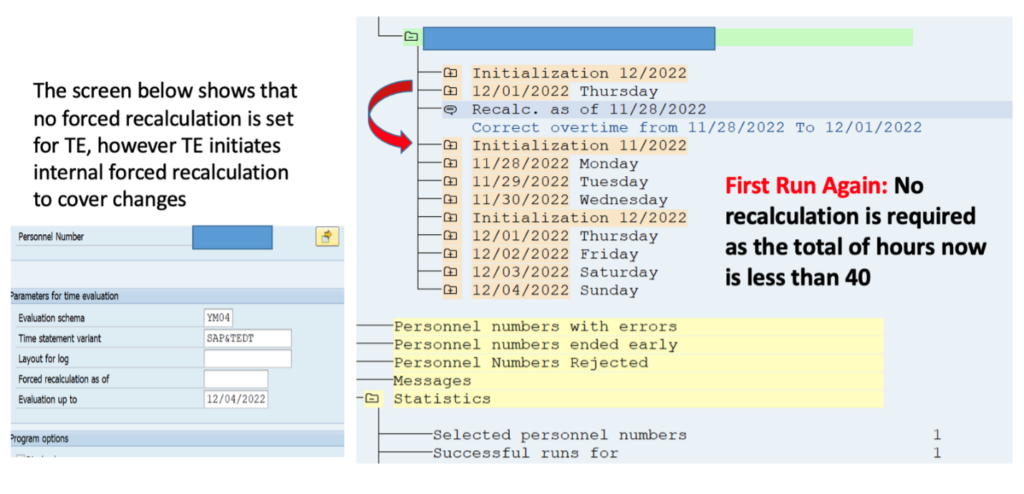
If there is change in master data on Thursday, the system immediately initiates IFR. The process then starts from the beginning and new first run starts. At the end of the work period, the system decides if there is a need for IFR based on new master data.

This configuration is separate, can be introduced on top of the existing solution, and is straight-forward.

Conclusion

The discussed solution resolves the problem of master data changes inside the recalculated time periods in when the internal forced recalculation is in place. It makes the additional Time Evaluation runs before payroll unnecessary and makes the results accurate for the current and previous payroll periods. The configuration is based on standard time types settings (that represent the checksums for day in questions) and can be easily applied to the existing time evaluation solutions.

[1] Operation GOTC can send time type to the beginning of the week defined in Planned working time infotypes 0007, to the beginning of Payroll period, to Monday (as the first day of the week), to the day defined by the feature LDAW and so on – pretty impressive operation! The only disadvantage of this operation is that it can send only one type and sometimes it is not sufficient – in this case two or more recalculations are required, and Time Evaluation sends different time types to make all calculations accurate.

[2] In SAP Mater Data changes are tracked in infotype 0003 (Payroll Status). If there are changes in absences, attendances, substitutions, planned working time, org. assignment as special field in Infotype 0003 is set to the earliest date of changes. Next time when time evaluation is run it starts with this date. After Time Evaluation this date is set to the date when Time evaluation was run (plus one day) so next time SAP Time evaluation starts with this date