Demand Driven Planning – Strategic Inventory Positioning – Step 1

⇨ SAP offers consulting solutions to enable strategic inventory positioning, the first step in demand-driven planning.

⇨ ‘MRP Monitor’, SAP's consulting solution, can be used to detect the ‘to-be’ buffered materials.

⇨ MRP Monitor can be used for materials, in addition to the multi-dimensional classification, to detect which parts are important/non-important

Step 1 – Strategic Inventory Positioning

In my last article, I gave an overview of the Demand Driven Planning logic in SAP ECC or SAP S/4HANA using SCM consulting solutions. Consulting solutions are small add-on tools that can be used in SAP to cover so called “white spots”. This article will focus on the first step in Demand Driven Planning, Strategic Inventory Positioning, identified by the Demand Driven institute.

To identify products that can serve as decoupling points, they need to be systematically evaluated and classified for example, according to the:

• Goods issue value
• Decoupled lead time
• BOM usage
• Variation in actual demand or consumption

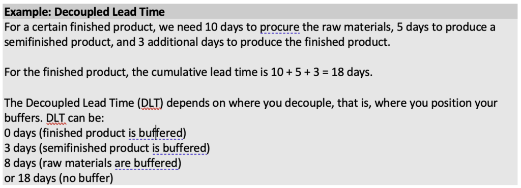
As a first step, decoupling points must be identified, and the decoupled replenishment lead time must be determined. To decide which materials produced in-house and externally procured are to be buffered, the lead time of the product must be compared with the delivery time accepted by the customer. When we talk about the lead time for a manufactured product, we typically think of one of the following two situations:

• Either at the time it takes to manufacture the product when all components are available, or in the other extreme.
• The longest BOM path requires that no components are available (cumulative lead time).

With the introduction of buffered (stocked) materials, the longest BOM path must be decoupled, that is, an attempt is made to find a golden middle path from the two situations mentioned above. DDP refers to this as Decoupled Lead Time (DLT).

Different criteria can be used to identify the materials that can serve as decoupling points. This includes the following three classification methods:

• EFG Analysis (Replenishment Lead Time Analysis)
• XYZ Analysis (Consumption Analysis)
• PQR Analysis (BOM Analysis)

The results of these classifications can be used to identify products that should be relevant for demand-driven replenishment. All three classification methods will be discussed in detail another article of this series.

However, there are other criteria to find decoupling points. This includes, for example:

• Accepted market delivery time
  The accepted market delivery time is the maximum delivery time accepted by the customer, that is, the time between the customer’s order and the delivery to the customer.
• Requirement Visibility Horizon
  This is the horizon in which demands are visible.
• Maximum replenishment lead time
  The maximum total replenishment lead time ensures that even if the buffer calculated based on the accepted market delivery time is not sufficient, the maximum total replenishment lead time does not exceed.

If we now assume an accepted market delivery time of 20 days for our sample material, material 2SFG_MH_100 must be used as a decoupling point (Image below).

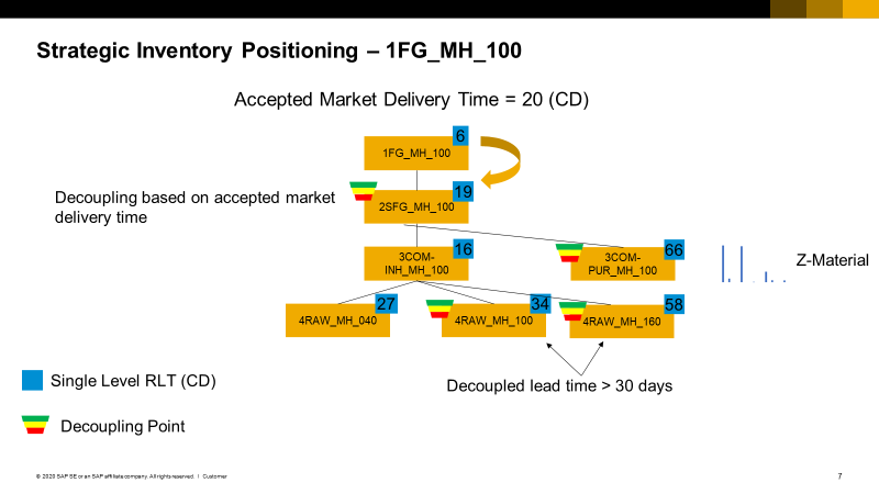
Decoupling According to Accepted Market Delivery Time

The delivery time of the finished product of 6 days is sufficient to cover the accepted market delivery time. This means that the finished product does not have to be buffered. If we add the 6 days for the finished product and the 19 days for the semifinished product, we get to 25 days, which is greater than the accepted market delivery time. Thus, the semifinished product must be buffered to meet the accepted market delivery time.

This determination can be performed using transaction /SAPLOM/SLM (BOM Analysis) (Image below).

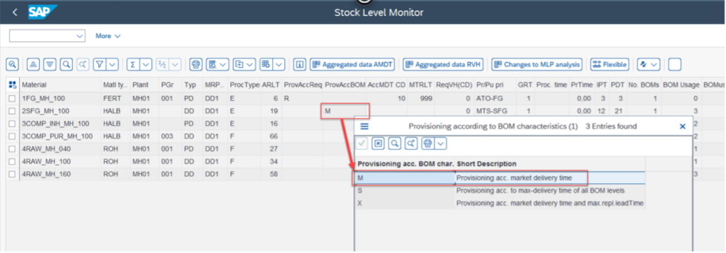
Result of BOM Analysis

The material 2SFG_MH_100 has been determined as a decoupling point and in the Prov. Rep. BOM (stocking level according to BOM) with “M”. “M” here means that the stocking has been determined according to the market delivery time.

Next, transaction/SAPLOM/MRP is used to perform a classification according to the consumption fluctuation (XYZ analysis, see unit 3, “Material Classification/Material Segmentation”). The result can be seen in picture.

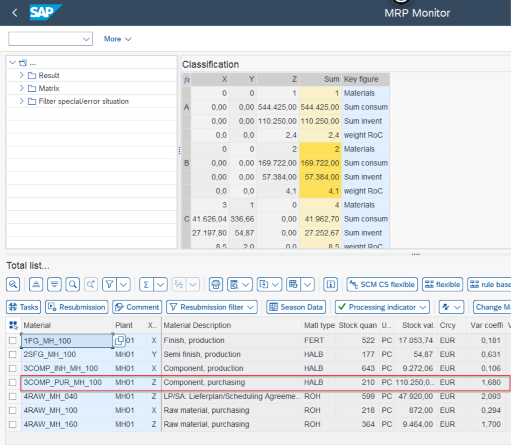
Result of XYZ Classification

The externally procured component 3COMP_PUR_MH_100 is flagged as a Z material, which is a sporadic material and should be buffered.

Furthermore, an analysis can be performed according to the replenishment lead time, so that materials with, for example, more than 30 days replenishment lead time should also be buffered. This gives an overall picture of the materials that are to be buffered for the production of the finished product (Image below).

Result of the decoupling points for the sample material

Material 2SFG_MH_100 is buffered according to the accepted market delivery time, material 3COM-PUR_MH_100 is buffered according to its classification as Z material (sporadic consumptions), and materials 4RAW_MH_100 and 4RAW_MH_160 are buffered according to their long replenishment lead time. Now that the decoupling points are fixed, the next step is to calculate the buffers.

The next article will discuss buffer level and calculation.