Demand Driven Planning – Dynamic Adjustment – Step 3
Key Takeaways
⇨ With SAP consulting solution safety stock and buffer simulation, buffers can be dynamically adjusted according to the demand driven planning logic in SAP ECC 6.0.
⇨ Using dynamic adjustments of buffers, organizations can react quickly to market changes or supply interruptions.
⇨ Demand driven planning can be used for MRP planning in SAP ECC 6.0 or extend the demand driven logic on S/4HANA.
In the series of articles on demand driven planning with SAP ECC, we covered the first two steps in Demand Driven Planning, Strategic Inventory Positioning, and Buffer Management (buffer profile and buffer level determinations). This article will focus on the third step identified by the Demand Driven Institute, called Dynamic Adjustments.
In DDP, buffers are adjusted dynamically if certain general conditions change. Below are some examples of changing conditions and their effect on DDP.
- Change in Average Daily Usage (ADU)
Buffers must be recalculated if the average daily usage changes and changed daily, weekly, or monthly depending on the analysis period. If the average daily usage is calculated based on the last three months, the key figure should be checked daily or weekly. If the base is more than six months, it is sufficient to recalculate the key figure monthly. With the SAP add-on safety stock and buffer simulation (TCODE: /SAPLOM/SSS), demand influencing factors like the average daily usage can be changed (Image 1).
Explore related questions

Image 1: Dynamic adjustments – Demand Adjustment Factor
- Change of Decoupled Replenishment Lead Time
It is often the case that components in the BOM must be replaced or that the delivery time of existing components changes. This can influence the decoupled replenishment lead time and, therefore, must be recalculated. Since this affects the buffer calculation, the buffers must also be recalculated. Decoupled replenishment lead time can be calculated with transaction /SAPLOM/RLT (Image 2).
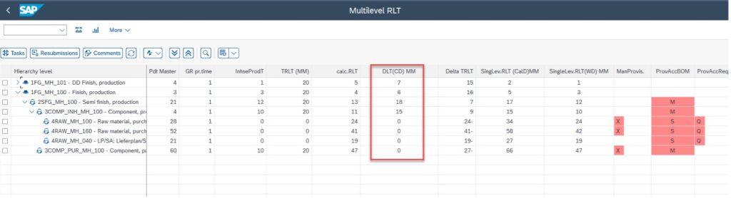
Image 2: Buffer Profiles and Levels – Calculation Decoupling Lead Time
With the SAP add-on safety stock and buffer simulation (TCODE: /SAPLOM/SSS), supply influencing factors like the decoupled lead time can be changed (Image 3).
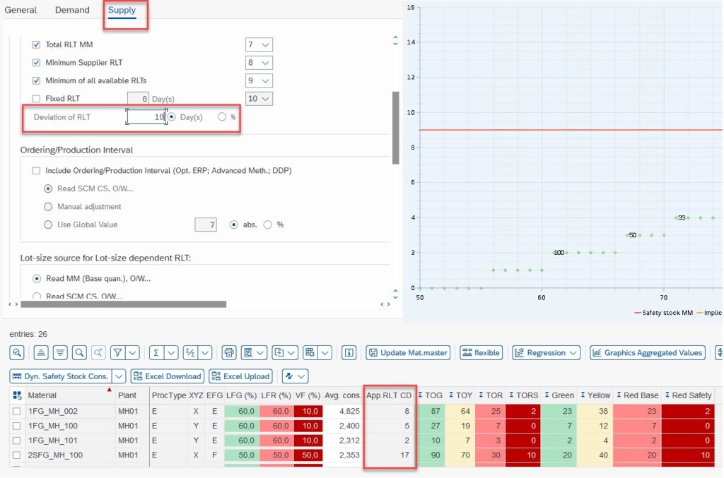
Image 3: Dynamic adjustments – Lead Time Adjustment Factor
- Change of Minimum Lot Size
The change of the minimum lot size that the supplier triggers has an impact on the green zone, so a buffer level calculation needs to be triggered in this case too.
- Change of EFG classification
If the replenishment lead time of a material changes, it may be necessary to assign a new buffer profile to the material.
- XYZ Classification Change
If the consumption or demand of a material changes or fluctuates, for example, if the consumption variability of a material increases, then a new buffer profile must be assigned to the material and buffers must be recalculated. MRP Monitor (Transaction /SAPLOM/MRP) is used to recalculate the variability and assign new buffer profile to the material (Image 4).
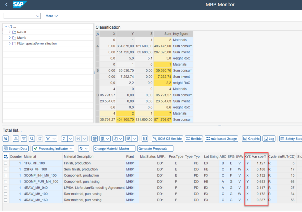
Image 4: Buffer Zones External Variability – Demand
Automatic adjustment is sufficient for most cases. However, it may be necessary to adjust the buffers manually when reacting to abnormal demand changes, for example, changed product lifecycle (phase-in, phase-out), marketing promotions, or seasonality.
The next step is DDP (MRP) planning in SAP S/4HANA or the SAP ERP system. This will be explained in the next article in our series on demand driven planning on SAP ECC.