Payroll schemas and rules are the bridge between HR Master Data and Payroll results. Creating that bridge is similar to writing programs and performing table configuration. Rules and schemas can be a confusing process for those who are not familiar with the concepts. Configured correctly, they can lead to a stable payroll calculation. Done incorrectly, they can produce difficult errors. In the first article of a two-part series, the author illustrates the basic principles of the payroll schema and rule process with the example of a cost of living allowance
Payroll schemas and rules are the bridge between HR master data and payroll results. Creating that bridge is similar to writing programs and performing table configuration. Rules and schemas can be a confusing process for those who are not familiar with the concepts. Configured correctly, they can lead to a stable payroll calculation. Done incorrectly, they can produce difficult errors.
This two-part series aims to familiarize you with the payroll schema and rule process. In this article, I’ll illustrate the basics with the example of a cost of living allowance (COLA) that I want the system to automatically calculate and pay to employees. I’ll present five COLA examples to show how the rules and schemas are applied.
For a download of background information on basic wage type processing concepts such as the relationship between a schema and a rule and for more detail for the examples that follow, click here: download. This series won’t make anyone an expert – the subject is too complex and broad to master without practice and experience – but it will get you started in the right direction.
Functions for Processing Wage Types: The two primary tables in payroll calculation are the Input Table (IT) and the Result Table (RT). Wage types in those tables are processed with functions Process Input Table (PIT) and Process Result Table (PRT). Each loops through the table and executes a rule for every wage type. Each function also has an Output Table (OT). When the function is finished, it returns the OT back to the payroll driver. I will use the PIT function for examples.
Calculating Values and Saving the Results: Each wage type has three fields you can calculate, named “number,” “rate,” and “amount.” Operations MULTI and DIVID can multiply and divide two fields and store the results in another field. After you multiply and divide, you save the results using the ADDWT operation. ADDWT copies the wage type in the header row to another table. You can copy it using the same or different wage type name. SUBWT does the same thing, except it multiplies the number and amount by -1 before copying.
Example 1: Calculating a COLA Wage Type
In my first example, COLA is paid at 15 percent of base pay. The base pay wage type is 0BAS and COLA is 0COL. In rule ZUA1, you process only wage type 0BAS. You execute rule ZUA1 from schema ZUA2 (a copy of standard schema UAP0), using the PIT function with parameter 2 blank, and parameter 3 as NOAB.
Figure 1 shows the calculation logic for rule ZUA1. For wage type 0BAS, four operations are processed:
- ADDWT *: copies the current wage type (in the header row) to the IT, keeping the same wage
type identifier 0BAS.
- NUM=0.15: sets the value of the wage type’s number field equal to 0.15
- MULTI ANA: multiplies the amount field by the number field and stores the result in the amount field
- ADDWT 0COL: copies the current wage type (0BAS) to the IT and renames it 0COL
Figure 2 shows the IT table after rule ZUA1. The wage type 0BAS is $2,000, Wage type 0COL appears with an amount of $300, and 0.15 is in the number field.

Figure 1
Calculation logic for rule ZUA1

Figure 2
IT table after calling rule ZUA1
Making Decisions in Rules
Decision Operations: Payroll rules allow you to perform conditional processing using decision operations. Think of decision operations as a type of “case” statement whereby you perform various operations for each value of a data element. Two of the most common decision operations are OUTWP and VAKEY. OUTWP makes decisions based on data elements from the employee’s infotypes 1, 7, and 8. VAKEY gives access to a variety of data elements, including the current payroll period and year, leave year, off-cycle reason and category, and some bank transfer specifications.
Working with the Variable Key: Decision operations place their data values in the rule’s eight-character variable key. When it finds a match between a line’s variable key and the decision operation’s data value, that line is executed. If it does not find a match, the decision operation resets the data value to the wildcard character “*” and takes another look to find a match. If it doesn’t, the employee is rejected from payroll with an error message.
Example 2: Restricting COLA to Specific Groups of Employees
The previous example paid 15 percent COLA to every employee. Let’s refine that by saying only employees in employee subgroup PS and personnel area ACAF can receive COLA. Figure 3 shows rule ZUA3, where you have a nested decision. You tell the OUTWP operation that you want to put the value of the employee’s personnel area (i.e., PLANT, the former term for personnel area) in the variable key. If the employee is in personnel area ACAF, then you look at which employee subgroup they are in (OUTWP operation with the PERSB option). If they are in employee subgroup PS, then you calculate COLA.
For employees who are not in personnel area ACAF, or who are in ACAF but not employee subgroup PS, you perform the ADDWT * operation. This copies wage type 0BAS from the header row to the IT. If you don’t do this, that wage type is dropped from the payroll calculation.

Figure 3
Rule ZUA3 — a nested decision
Working with Wage Type Values
Amount, Rate, and Number Fields: The next three operations are small but powerful – AMT, RTE, and NUM. They work the same, but affect different fields of the wage type. In addition to setting a field to a literal value, they assign other values. The syntax for these operations can be a bit complicated, so it’s useful to refer to the system documentation. (Select the operation with your cursor and press F1 for help.)
Note!
Documentation for the function, operation, schema, and rule editors is available online at
https://help.sap.com. Click on
SAP R/3 and R/3 Enterprise, select your release level and language, and go to the
Human Resources>HR Tools section.
A common practice is to use these operations to assign the value of another wage type to the current wage type — for example, to set the amount field of the current wage type equal to the amount field of wage type “x” in the IT. You can also assign it to the number of days or hours in the payroll period or the number of absence hours in the period, among others. The value of constants from view v_t511k can also be assigned. There are several operators for these operations (Table 1).
| Operator |
Description |
| = |
Assign value to field |
| - |
Subtract value from field. If the amount field equals 10, AMT-8 will leave it at 2. |
| + |
Add value to field |
| / |
Divide field by value |
| * |
Multiply field |
| < |
Set field to the minimum of its current value or the operand. If the amount field is currently 10, AMT<8 sets it to 8. |
| > |
Set field to maximum value |
|
| Table 1 |
Commonly used operators |
Making Decisions Based on a Value: The other use for these operations is making decisions. The “?” operator compares the current value of the field to another value, and places “=,” “<,” or “>” in the variable key. For example, if the amount is 10, then AMT?8 places the “>” sign in the variable key.
Example 3: Bracketed Calculations and Flat-Amount Override
Let’s change the COLA calculation from a flat 15 percent to one that changes with the amount of base pay — 15 percent for base pay up to $1,500, 10 percent for $1,500 to $2,000, and 5 percent for more than $2,000. To handle exceptions that always occur in payroll, let’s say that if someone enters the COLA wage type 0COL via master data with a fixed amount, you pay that amount instead of using the calculation logic.
Since not enough room is left in the variable key, you put the new logic in another rule and execute it only for employees in personnel area ACAF and employee subgroup PS, as shown in Figure 4. I’ve changed the line type to P, which tells the PIT function you are going to call a sub-rule on that line. Operation PCY calls rule ZUA5 and then returns to ZUA4.

Figure 4
Rule executed only for employees in personnel area ACAF and employee subgroup PS
Rule ZUA5 calculates the COLA amount. In Figure 5, line 10, set the amount field equal to the value of wage type 0COL in the IT, and compare that amount to zero. If someone had entered wage type 0COL in infotypes 14, 15, 267, or 2010 this period, you would have that wage type in the IT. In that case, the amount is greater than zero, so line 20 is executed (the “*” condition, since there is no “>” case in the rule). Remember that wage type 0BAS is in the header, and it’s that wage type’s amount that you just set to the value of 0COL. Operation FILLF resets the amount (A), number (N), and rate (R) fields of the header row back to their original values. After that, you copy 0BAS back to the IT.

Figure 5
Rule ZUA5 calculates COLA amount
If wage type 0COL has an amount of zero, or if it doesn’t exist in the IT, line 30 is executed. You again use FILLF to restore the amount field and then compare it to the value of $1,500. If it is less than $1,500, line 70 is executed. Compare the amount field to $2,000, and if it is less than that, execute line 60. Otherwise, you know the value is $2,000 or greater, and use line 50 to calculate COLA.
When payroll is run, you can see the decision logic for the new rule in the payroll log (Figure 6). In the processing section for rule ZUA4, it determined the employee was in personnel area ACAF and employee subgroup PS, so it called subrule ZUA5. It tested the value of 0COL and found it was zero. It calculated wage type 0COL based on the value in wage type 0BAS and then returned to rule ZUA4, where it ended.

Figure 6
Decision logic in payroll log
Figure 7 shows wage type 0COL entered on infotype 2010 with an amount of $150. The amount doesn’t show in the processing section, but you can see the different logic that was used because there was something in the amount field.

Figure 7
Logic when amount is entered
Making It Date-Effective
Processing Classes: The COLA calculation is getting closer to a real example, but a couple of items are missing. Many calculations like this are done on a set of wage types, not just a single one like base pay. Processing classes can specify which wage types are subject to the COLA calculation. Customers can create their own processing classes, starting with class 99 and working down. The processing class value of a wage type can be read in the rule, which can subject it to certain calculations and other processing.
Processing classes are a preferred way to get wage types into a rule, instead of hard-coding them as in the previous examples. I used hard-coding for the wage types to make the first examples easier to understand. If the COLA policy is eliminated some time in the future, then how do you stop calculating it? Payroll rules have no effective dates, so if you remove the logic in the rule and a retrocalculation happens, you will not calculate COLA at all. The system would determine that employees who received COLA in the past were overpaid, and it would take that money back from the current payroll. However, there are effective dates on wage types and the processing class values assigned to them. If COLA were discontinued, you would only have to make a date-effective change to the wage type’s processing class.
Payroll Constants: What if COLA rates or wage brackets change? Those numbers are hard-coded in the rules. A better practice is to put those values in the payroll constants table t511k. Those constants are date-effective, so if the rates or wage-brackets change in the future, you just update view v_t511k.
Example 4: COLA with Date Flexibility
For this example, I’m moving the COLA wage brackets and rates into v_t511k constants, as shown in Figure 8. With this new calculation structure, you can change which wage types are subject to COLA, the wage brackets, and the rates by effective dates. It requires a little extra time for configuration (15 minutes for me), but it also provides flexibility and stability. Based on my experience, calculations like this change over time, so configuring the system to account for this makes sense.
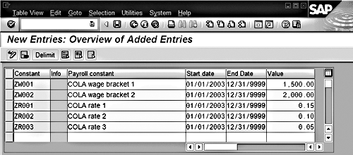
Figure 8
Moving the COLA wage brackets and rates into v_t511k constants
As shown in Figure 9, you can create Processing class 90 to specify which wage types are subject to the COLA rate. Then in the wage type view v_512w_o, you assign wage types 0BAS to value 1 in processing class 90.

Figure 9
Creating Processing class 90
The payroll rules change a bit, too. In schema ZUA2 where you call the rule, you use a different syntax. Parameter 2 was empty in the previous examples; now you set it to P90, which tells PIT to send all wage types to the rule, along with their processing class 90 values.
In rule ZUA6 (Figure 10) there is a new decision operation called VWTCL. It was used to put the value of processing class 90 in the variable key. If processing class 90 for the current wage type has a value of 1 and the employee is in personnel area ACAF, then you execute rule ZUA7.

Figure 10
Decision operation called VWTCL places Class 90 in the variable key
In ZUA7 (Figure 11), you make a decision on the employee’s employee subgroup, and if it is PS, you continue with the calculations. The logic from this point is the same as in rule ZUA5, except you use constants instead of literal values.
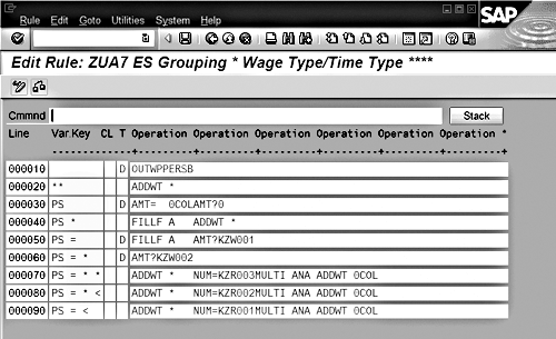
Figure 11
Using constants for the COLA wage brackets
Wage Type Splits
What Are Splits and Why Do I Need Them?: A wage type split is an attribute of a wage type that links it to another piece of data in payroll results. For example, if an employee changes cost centers in the middle of the pay period, R/3 splits certain wage types, linking one part to the first cost center and the other to the second. That is how you know how much to charge each cost center when running the posting to FI/CO. Other splits link a wage type to a tax authority, a benefit provider, and so on.
Figure 12 shows an RT result for Test Employee. The heading for the RT shows the splits that could exist (i.e., A, AP, C1, C2, C3, etc). See the download section at the bottom of the article for more material that describes some of the frequently used splits. If a wage type has no value for a split, there is no link.
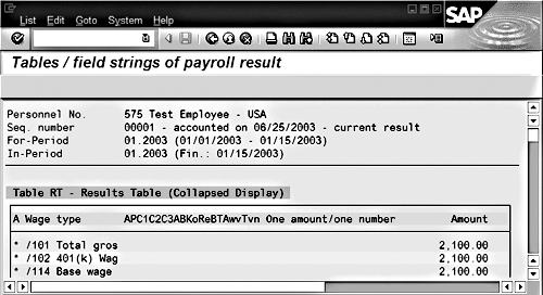
Figure 12
Sample RT result
Splits in Rule Processing: Splits cause confusion because a rule may have been set up so that it expects only one occurrence of a wage type. The split causes two occurrences, though, and custom rules need to consider that possibility. For example, the test employee transferred in the middle of period two, so two cost centers are charged. Since COLA is calculated on wage types, and there are two in this example, two COLA wage types result. The current calculation logic doesn’t work because it does not consider the total base pay for the whole period. The IT has two wage types 0BAS, as shown in Figure 13. The first is calculated at a COLA rate of 0.15 and the second at 0.10 because those are the wage brackets they fall into on an individual basis. However, together for the whole period, they add up to $2,000, which falls into the 0.05 COLA rate.
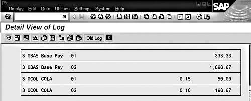
Figure 13
View of two wage types
The rule also doesn’t work for mid-period transfers when COLA is entered with an override amount. In period 3, there was another transfer plus a $150 COLA override was entered on infotype 2010. Figure 14 shows the incorrect result. How did this happen?

Figure 14
Incorrect result after mid-period transfer
When rule ZUA7 processes the first wage type 0BAS, it looks for wage type 0COL in the IT, with the same corresponding value for all the split indicators. So for wage type 0BAS with split AP = 01 and split A = 3, it finds wage type 0COL with split AP = 01 and split A = 3 (wage type 0COL was entered in infotype 2010 on the first day of the pay period and was assigned to the first AP split of 01). But when it processes 0BAS with split AP = 02 and split A = 3, it doesn’t find a matching 0COL wage type, so it returns a value of zero. When rule ZUA7 sees a value of zero for 0COL, it processes the automatic COLA calculation.
Example 5: Calculate COLA with Splits
One of the challenges with the COLA calculation is that the wages must be cumulated regardless of splits, with COLA based on the total amount. To do this, break the calculation into three rules instead of two. The first two rules, ZUA8 and ZUA9, build the COLA wage base in a new wage type 9COL. ZUA8 is a copy of ZUA6, and ZUA9 is shown in Figure 15. A new operation – ELIMI – eliminates the split indicators on the wage type in the header row. Copy that wage type to 9COL to build a wage base for COLA that goes across all splits in the payroll result. Now you can assign more than one wage type to the COLA wage base using processing class 90, value 1. Any wage type with the specification cumulates to 9COL.1
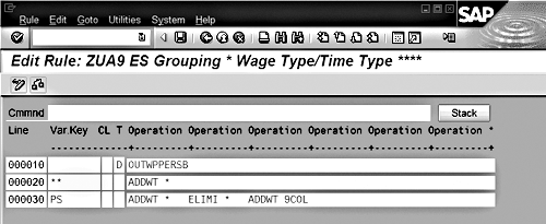
Figure 15
Rule ZUA9 – build COLA wage base
The next rule is ZUAA. It calculates the COLA amount, as shown in Figure 16. For each wage type that cumulated to the COLA wage base (processing class 90, value 1), you look for a corresponding wage type 0COL. Wage type 0COL in this case is entered on infotype 14, and its processing class 10 has been changed to a value of 1. This allocates it across the payroll splits in the same way as wage type 0BAS. If you do not have an override wage type 0COL, eliminate all the splits and look for an amount in wage type 9COL in the IT (line 050), the wage type built in the preceding rules ZUA8 and ZUA9. Compare that amount to the constants to see which wage bracket the COLA allowance falls into. Once you find the bracket, set the splits back to their original values with RESET * and calculate COLA as in previous rules. Figure 17 shows the results, with COLA calculated for each occurrence of 0BAS. Not shown is wage type 9COL, which has a value of $2,000 and no splits.

Figure 16
Calculate COLA amount based on COLA wage base
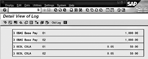
Figure 17
COLA calculated for each occurrence of 0BAS
Steve Bogner
Steve Bogner is a managing partner at Insight Consulting Partners and has been working with SAP HR since 1993. He has consulted for various public, private, domestic, and global companies on their SAP HR/Payroll implementations; presented at the SAP user's group ASUG; and been featured on the Sky Radio Network program regarding SAP HR.
Steve will be presenting at the upcoming HR Payroll Seminar November 7-8 in Chicago and November 27-28 in Orlando. For information on the event, click
here.
You may contact the author at sbogner@insightcp.com.
If you have comments about this article or publication, or would like to submit an article idea, please contact the editor.