Companies sometimes want to perform long-term capacity planning in a tight production schedule with different production lines allocated to product groups. This kind of situation occurs in the consumer products industry where companies manufacture products or product groups on dedicated production lines in specific time periods during a month or quarter.

Based on the sales volume, they manufacture the products frequently— for example once a month or quarterly — by accumulating the demand. One of my clients has a typical production schedule driven by product groups (based on their sales volume) on dedicated production lines in specific time periods. This client wanted to implement SAP Advanced Planning & Optimization (SAP APO) Supply Network Planning (SNP) and integrate its existing SAP ERP production planning into SAP APO.

The client wanted to create a production schedule based on the actual shop floor schedules, review the long-term capacity plan with SAP NetWeaver BW metrics, fine tune its capacities, and, finally, generate a feasible production schedule for manufacturing plants. I assume that the reader has some prior knowledge about SAP APO master data, SAP ERP-APO core interface (CIF), the setup for new SNP planning areas, SNP planning books, and macro elements.

Details About Business Needs

My client, a global company, performs forecasting in SAP APO Demand Planning (DP). The forecast output feeds into SAP APO SNP for supply planning. Demand from the client’s 10 involved countries is aggregated and fed into manufacturing plants. The manufacturing lines are dedicated to different product groups only in certain weeks in the plant calendar, based on sales volume. For more detail, see my article, “Use SAP APO SNP to Improve Runs for Products with Recurring Time Constraints.” That article explains the process we followed to select this option and the functionality we implemented for this client.

Figure 1 shows the business process flow of the solution I discuss, including the sequence of macros and their inputs and outputs.

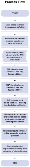
Figure 1

Business process flow of the SAP APO solutions discussed in this article

Elements for Configuration

Below is a detailed explanation of the configuration we implemented in the system.

Mapping Time-Stream IDs to the Product Master

Step 1. Map the shop-floor, product-group-based planning calendars into different time streams in SAP APO. All the time horizons have been divided by naming them weekly, biweekly, and monthly time-stream stamps. Every week has been allocated to the time-stream ID as shown in the spreadsheet in Figure 2, which lists all the weekly time buckets in a year and groups them based on time stream with an X in the buckets.

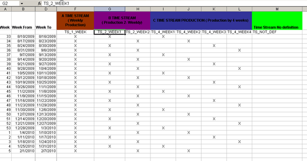
Figure 2

Weeks mapping to the different time-stream-based calendars

Step 2. Create detailed time-stream IDs with the relevant weekly or biweekly time windows in the SAP APO planning system (Figures 3 and 4). Use transaction code S_AP9_75000138 (Maintain Planning Calendar [Time Stream]) or follow menu path SAP Menu > Advanced Planning & Optimization > Supply Network Planning > Environment > Current Settings > S_AP9_75000138 - Maintain Planning Calendar (Time Stream). Enter the name of the time-stream ID in the transaction, enter years in the past and future in the header data, and enter the time buckets manually in the From-date and To Date fields, and then save the time stream. 

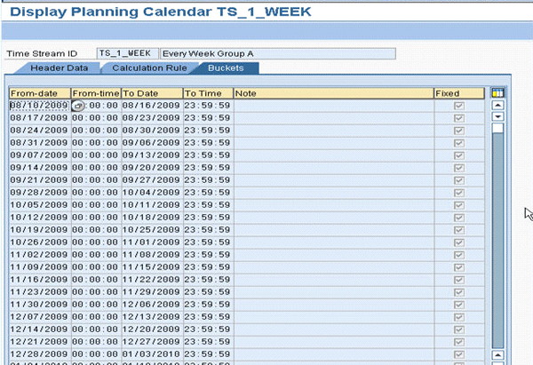
Figure 3

Weekly time-stream calendars created in SAP APO as time-stream IDs

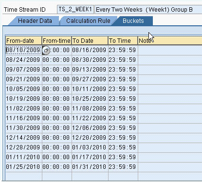
Figure 4

Biweekly time-stream calendars created in SAP APO as time-stream IDs

The intent is to have only the periods that you entered in the time-stream ID as active periods for production.  

Step 3. Enter the time-stream IDs that you just created into the SAP APO product master by using transaction /SAPAPO/MAT1 – Product (Figure 5). These time-stream IDs have been stored in the product master as additional fields so that they are easily accessible to the SNP planning book macros. Enter the respective product and location, and enter the time-stream ID under the Production Frequency field near the bottom of the screen. The macro logic is to read the time-stream ID from the product master, determine the planning periods based on the active time buckets, and create the production planning time periods. Then, based on these time periods, SNP heuristics creates the production planning receipts in these time buckets.

Figure 5

Time-stream ID calendars are attached to the product based on the product group

SNP Planning Area and Planning Book Changes

As the client wanted to implement the entire solution within SNP and to use SNP heuristics as the algorithm for planning, I had to change the SNP planning area and SNP planning books to get the right results from SNP heuristics planning.

We copied standard SNP planning area 9ASNP02 into a new planning area. Using transaction RSA1 BW, I created new key figures: Y_EXTRA1, Y_EXTRA2, Y_EXTRA3, Y_FREQNCY, Y_PDEMAND, and Y_PLNPERD. I added the new key figures to the planning area so that production frequency logic could be built in the new SNP planning area and planning books. To do this, use transaction /SAPAPO/MSDP_ADMIN – Administration of Demand Planning and Supply Network Planning or follow menu path SAP Menu > Advanced planning and Optimization > Supply Network Planning > Environment > Current Settings >  /SAPAPO/MSDP_ADMIN – Administration of Demand Planning and Supply Network Planning. Right-click your SNP planning area and choose the option to change the planning area, which then leads to the screen in Figure 6. The primary purpose of adding these extra key figures is to use them in the different production frequency-based planning receipts generation logic. For example, a macro reads the product master time-stream field and designates the time periods as active or not active in the Y_FREQUENCY key figure so that SNP heuristics knows where to create the planning receipts.

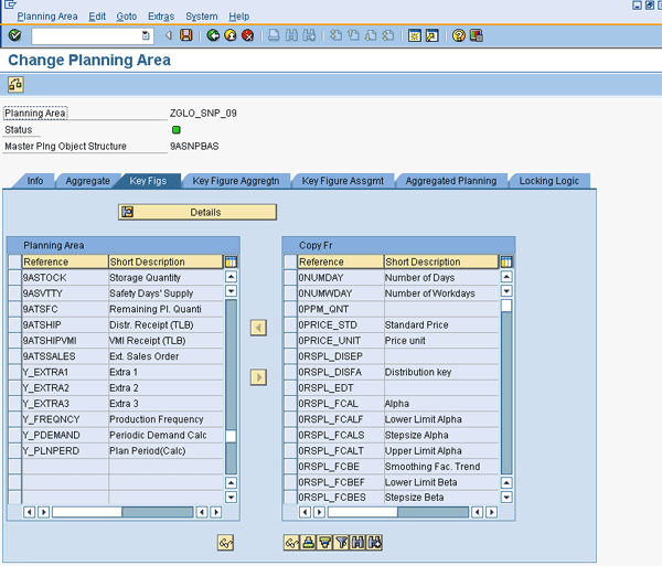
Figure 6

SNP planning area copy with new key figures added

To view the data, I created separate SNP planning books by using the standard APO planning books creation transaction /SAPAPO/SDP8B — Define Planning Book. This step allows you to create the planning results based on production frequency and to view the resource capacity information in the planning book as the resource available capacity versus resource capacity consumed by the planning results.

Figure 7 shows a sample view of the planning book and the different key figures. I made provisions to enter the buffer stock requirements in the planning books key figures, such as production planning changes (PPC). The PPC key figures can accommodate regular production planning changes or allow for extra buffer stocks to accommodate any future sales order spikes. Safety-stock-related demand, such as PPC, rolls up into the total demand for further calculation purposes in the planning book.

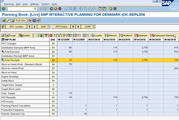
Figure 7

SNP planning book view

Digging Into the Macros

The SNP planning book and macros have been configured so that the system considers the production planning frequency (Figure 8). As shown earlier, the product master has the time stream saved in its master data fields. The macro’s logic arranges the demand so that SNP heuristics looks at the total demand and total receipts together with the production frequency active periods, and then SNP heuristics creates the production planning proposals to match the production frequency.

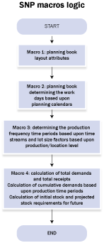
Figure 8

Flow process of SNP macros logic

Macro 1 — Layout Attributes

Macro 1, shown in Figure 9, locks the planned key figures at an aggregated level and leaves them open for input only at the Product/Location level. In this first macro, all the related key figures — including PPC Changes, Production (Planned), and Distribution Receipt (Planned) — are locked when they are not at the Product/Location detailed level. They are open for editing only when they are at Product/Location level. By using these key figures, the later macros formulate the logic for the planned receipts time buckets creation.

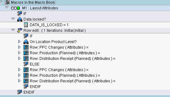
Figure 9

Unlocking key figures at the Product/Location level and locking them at all other levels

Macro 2 — Work Day Determination

Macro 2 determines how many work days there are in each period based on the location calendar by reading the location master. The macro calculates the bucket week days in a particular time bucket in the planning book (Figure 10).

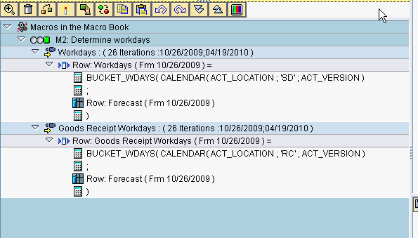
Figure 10

Determining the work days by calendar/period

Macro 3 — Production Frequency

In Macro 3, the step for Time Steam Definition: TS reads the production time frequency from the product master and determines the planning period, and the step Minimum Lot Size: ML determines the minimum lot size for planning purposes (Figure 11). The macro is only executed at the Product/Location level.

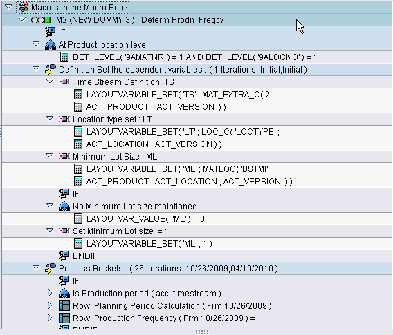
Figure 11

The first step determines calculation-dependent variables

Macro 3 reads the time stream from the SAP APO product master and evaluates the time stream. The intention of reading the time stream is to determine whether a period can be planned, as the client wanted to produce certain product groups only in certain periods. Based on this time stream, the system determines which periods can be planned and which periods cannot.

In Figure 11, under Definition Set the dependent variables, the system determines the time stream, location type, and product lot size information for further processing in the dynamic memory tables and variables. If there is no lot size found for a particular product and location, then a default value of 1 is used for the lot size. 

Based on the product master field that I stored earlier, the second step in macro 3 (Process Buckets) reads the time stream and determines the bucket week days for the processing week period (Figure 12). Based on the time-stream configuration, if the system determines the number of working days as more than zero in that particular week, the system stamps that week as a work week for that product/location combination.

The macro allows SNP heuristics to create further planning receipts in that particular weekly time bucket. In the step Row: Production Frequency, the logic system populates the production frequency row with the minimum lot size so that the particular period is marked for planning.

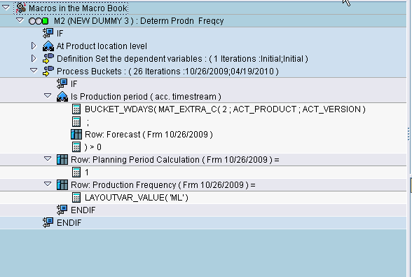
Figure 12

Determine the production periods based on the time-stream calendars

Macro 4 — Demand Calculation

Macro 4 adds the different demands and plans based on the production frequency time periods (Figure 13). As an output from this macro, the consolidated demand feeds into SNP heuristics so that heuristics creates the planned orders based on the planning periods.

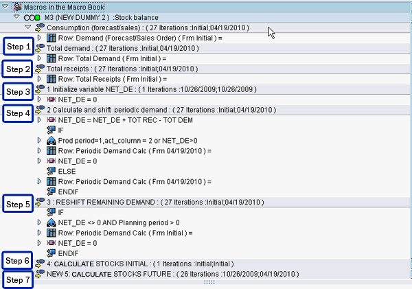
Figure 13

Steps to calculate the total demand and total receipts and accumulate the demand based on production periods

The system takes the following steps automatically as shown in Figure 13:

Step 1. The lines Total demand and Row: Total Demand add the related demand key figures from the SNP planning book so that the system can determine total demand numbers.

Step 2. The lines Total receipts and Row: Total Receipts add the related supply key figures from the SNP planning book so that the system can determine total supply numbers.

Step 3. The line Initialize variable NET_DE initializes the net cumulative demand variables and accumulates the demand backwards to each planning period based on the production periods that the system determined earlier.

Step 4 and Step 5: The lines Calculate and shift periodic demand and RESHIFT REMAINING DEMAND add the cumulative demands in each period based on the active planning periods determined by production frequency. These steps make the demands in nonactive planning periods added cumulatively to active planning periods. With these steps, the system determines the demand in each active planning period.

Let’s continue the review of automatic steps for macro 4 in Figure 14:

Step 6 and Step 7: CALCULATE STOCKS INITIAL determines the initial stock in the system and, based upon the total demand, CALCULATE STOCKS FUTURE projects the stock which has to be on hand in future periods.

Note how the subrows under CALCULATE STOCKS INITIAL and CALCULATE STOCKS FUTURE determine the stock on hand projection calculations for initial and future periods so that SNP heuristics can read this demand and create the related planned receipts in the future.  

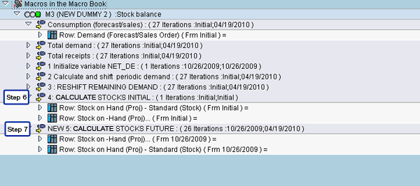
Figure 14

Calculate the stock on hand and the projection for initial and future periods

Figure 15 shows the desired output of macro 4 in the interactive SNP planning screen. Use transaction /SAPAPO/SNP94 – Interactive Supply Network Planning or follow menu path SAP Menu > Advanced planning and Optimization > Supply Network Planning > /SAPAPO/SNP94 - Interactive Supply Network Planning. In the SNP planning book, when the planner displays the product location from the SNP macros, the logic system displays the planning time periods in the Planning Period Calculation and Production Frequency key figures near the bottom of the screen in Figure 15. Based on the data from these key figures, SNP heuristics creates planning receipts in the planning book.

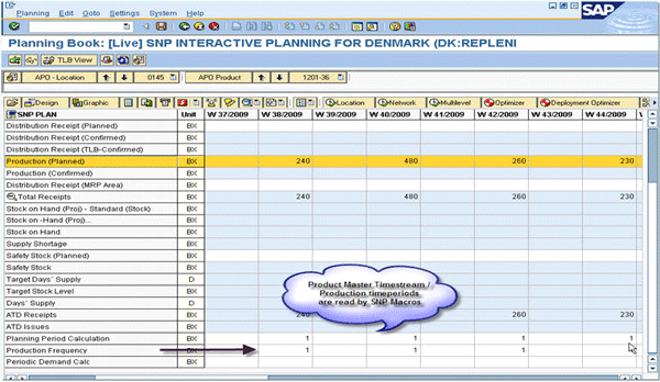
Figure 15

SNP planning book results from the SNP macros

SNP Heuristics Output Results

When a user invokes the location heuristics functionality, SNP heuristics creates the planned receipt proposals as indicated by the SNAP macro logic (Figure 16). For example, based on a biweekly time-stream calendar, SNP heuristics creates production proposals in week 38 (designated as W 38/2009 in Figure 16), skips week 39, and creates production proposals again in week 40.

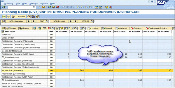
Figure 16

SNP heuristics compiles production time frequency for a biweekly production time-stream calendar

The SNP heuristics also uses the lot size definitions as defined in the product master as well as the planned safety stock.

SAP ERP-APO CIF Integration

Apart from the above changes in the product master additional attributes, all other master data follows standard integration between SAP ERP and SAP APO. All SAP ERP work centers have been created as SAP APO resources. Standard SAP ERP-APO CIF integration maps out multiple routings and alternative bills of material as production process models in SAP APO for planning purposes. SAP ERP Material Requirements Planning (MRP) performs component planning, and only finished goods planning is done in SAP APO. As the scope of this article is primarily to explain the production frequency-based configuration in SNP planning, I did not go into much detail in the SAP APO resource/PPM setup. Most of the SAP APO master data follows the standard SAP APO route. The planned orders have been directly integrated with SAP ERP and have been converted to production orders for execution by following standard CIF integration methods.

SAP NetWeaver BW Query

After the client completed the SNP planning run, I developed an SAP NetWeaver BW query planning results analysis by using the remote cube on the SNP planning area. Based on this query, users can conduct both macro- and micro-level planning run analyses. Figure 17 offers a sample view of this metrics-based analysis. It gives the available capacity and capacity consumption on each resource so that users have a clear understanding of how much production quantity has been planned and where the resources have been overloaded or underloaded. Users then can make any necessary adjustments.

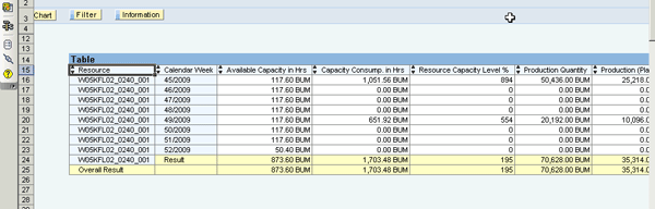
Figure 17

SAP NetWeaver BW query-based analysis of SNP planning results

You can run these queries in simulated and active versions so that planners can perform necessary adjustments. In SAP APO, you can create multiple planning versions to run SNP. Planning version 000 is the active version, which updates directly in real time from SAP ERP. Other copied versions do not receive automatic updates from SAP ERP. My client wanted to have a simulated copy of planning version 000 so that the company could plan offline without SAP ERP updating the copied version.