Data mining has gained in popularity recently, with many companies using some form of data mining algorithms to extract value out of terabytes of data stored in their SAP ERP systems. For example, you can use data mining algorithms to identify the source of a specific hardware problem in a laptop by analyzing millions of support tickets and searching for commonalities.

Association analysis is a data mining algorithm that enables you to identify sets of products that share strong sales relationships. However, many people are unsure about how to carry out association analysis. The following step-by-step guide shows you how you can use the Data Mining Workbench and Analysis Process Designer (APD) to perform association analysis. Specifically, I will take a look at a store that sells three products: a DVD movie, a Blu-ray movie, and a movie poster. By using association analysis, I can analyze how these three products relate to each other and which of them are potentially good candidates for cross-selling opportunities.

Preparation: Understand the Goals and Cleanse the Data

It is important to mention that taking the time to clearly outline the ultimate goal is crucial to any data mining exercise. Enterprises have accumulated enormous amounts of data over the years and without identifying the purpose or hypothesis ahead of time, it is easy to waste a lot of time and energy only to find yourself nowhere closer to finding the answer. Try to formulate the goal of the data mining exercise in a single concise sentence. For example, I could state that my goal is “to identify pairs of products that resemble strong and positive sales correlation, based on historical sales within the last year, to propose meaningful cross-selling items on our customer-facing Web site.”

After you determine the goal, you then need to spend time defining the exact data set that should be used for your analysis. In fact, this is typically where most of the effort lies when it comes to data mining. Having a good understanding of the related SAP business processes helps, so it can be beneficial to engage an SAP ERP business analyst at this point. The process of defining the relevant data set includes such points as the appropriate selection criteria, time horizon, as well as outlier correction.

Step 1. Create the Association Analysis Model

This model contains the rules used during association analysis. Use transaction RSDMWBor follow SAP Easy Access menu path Data Mining > Data Mining Workbench to create a new model. When you are in the Data Mining Workbench, open the Association Analysis node, right-click the Association Analysis algorithm, and choose Create Model (Figure 1).

Figure 1

Create the association analysis model

Provide the technical name and description for your new model. Leave the remaining settings as is and click the green check icon (Figure 2).

Figure 2

Provide the model name and description

In my example, I am going to analyze billing document line items that I have loaded into an SAP NetWeaver BI InfoProvider from SAP ERP to identify product association rules. I assume that I can uniquely identify each record in the InfoProvider by billing document and line item number, similar to table VBRP (billing document line items) in SAP ERP. Figure 3 shows the fields that I need to add to my association model to analyze billing document items effectively. Click the add icon to add each field.

Figure 3

Specify the association model fields

I created the first field, 0MATERIAL, with Content Type set to Item. This field identifies the object that represents actual products that are part of association analysis rules. The second field titled 0BILL_NUM has the Content Type Transaction. This field helps the model identify the key for each unique sale. In my example, I consider each individual billing document to be a separate unique sale. That way any materials that exist on a single billing document are considered as sold together. However, it can also be beneficial to perform association analysis at a sold-to or plant level, as opposed to billing document level, to identify common patterns across customers and stores.

Click the Parameters tab to continue configuring the new association model. Keep the default parameters shown in Figure 4. Typically, Minimum Support is set at 1% to 2% and the Minimum Confidence is usually between 40% and 60%. Although I will come back to the detailed explanation of how these measures are configured later, you can always refer to the “Important Terms” sidebar for definitions of the three most important measures in association analysis: support, confidence, and lift. Click the activate icon to save and activate the new association model.

Figure 4

Specify model parameters

Step 2. Create the Analysis Process

Now that I have created an association model it is time to provide this model with some data and produce results. SAP NetWeaver BI uses APD to link InfoProviders with data mining models. You can access APD by using the SAP Easy Access menu path Data Mining > Data Mining Workbench (transaction RSDMWB) and clicking the Analysis Process Designer button (Figure 5).

Figure 5

Access APD from the Data Mining Workbench

Once inside APD, click the create icon to create a new analysis process. Select the Generic application from the pop-up screen (Figure 6).

Figure 6

Create a new analysis process

First, specify a meaningful description for the new analysis process. My process contains three nodes:

• The definition of the InfoProvider that provides the necessary data
  
  
• A filter that restricts the data to the specific subset that I want to analyze
  
  
• The association analysis model node

Drag and drop the InfoProvider node to the analysis board as shown in Figure 7. Choose the InfoProvider that contains the transactional data for billing line items. This can be any standard InfoProvider. Note that the technical name of the InfoProvider in your SAP NetWeaver BI environment is likely going to be different from the one provided in Figure 7. Just make sure that the InfoProvider you choose contains the billing document number and the material specified on the individual billing document items.

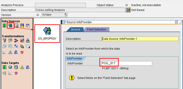
Figure 7

Choose an InfoProvider

Next, choose the fields that are going to be relevant to the following:

• The filter to apply to the data in the InfoProvider to select the data set
  
  
• The two fields necessary for the association model: billing document number and material number

Click the Field Selection tab in the Source InfoProvider window. In my example, I used the Calendar Year/Month and Plant characteristics for my filter and the Billing document and Material characteristics for the association model mapping (Figure 8).

Figure 8

Choose the relevant fields from the InfoProvider

Click the green check mark icon to return back to the analysis board (Figure 7). Now, drag and drop the filter icon to the board. Next, connect the InfoProvider node with the filter node on the analysis board as shown in Figure 9.

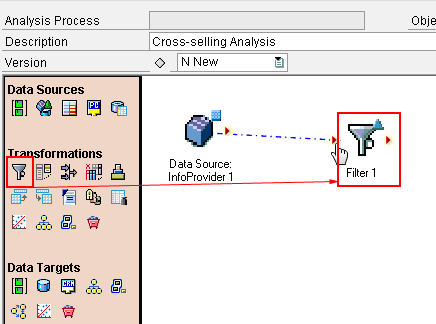
Figure 9

Add a filter node

Double-click the filter node to define the filter criteria. First, specify a meaningful description for the filter node. Then, choose the fields by which you want to filter. In Figure 10 I chose Calendar Year/Month and Plant as the filter fields.

Figure 10

Specify the fields for the filter

Next, go to the Filter Conditions tab and enter the values for your filter. For example, in Figure 11 I only select data for the month of November 2008 in plant 1704. I am keeping the data set small for the purposes of this article. You should leave your selection more open when performing association analysis against your real data.

Figure 11

Specify the filter values

Click the green check mark icon to complete the configuration of the filter node. For the final step, drag and drop the association analysis model node to the analysis board and connect the filter node to the association analysis model node as shown in Figure 12.

Figure 12

Add the Association Analysis model node

Double-click the Association Analysis node and specify the association analysis model that you created in step 1 (Figure 13). Click the green check mark icon to return to the analysis board.

Figure 13

Specify the association analysis model

Finally, double-click the field assignment icon between the filter and association analysis nodes to map the data set to the association analysis model. Click the arrow icons in the Method column next to each field in the Target Structure and map them as shown in Figure 14. Click the green check mark icon to return to the association analysis board.

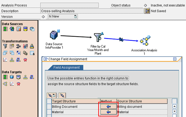
Figure 14

Map the fields to the association analysis target structure

At this point you are ready to activate and execute your analysis process. First, click the activate icon in the top-left section of the screen. Provide a technical name for the analysis process — in my example, I used AP_CROSS_SELLING. When the activation is complete, click the execute icon to launch the analysis process (Figure 15). The informational job log appears when the analysis process has finished executing. You should see no yellow or red lights if everything has executed successfully.

Note
I am executing the process in the foreground because my data set is fairly small. You might want to consider executing the analysis process in the background in the live environment with a larger data set, which you can accomplish by clicking the schedule job icon  in the top-left section of the screen in Figure 15.

Figure 15

Activate and execute the analysis process

Step 3. Review the Results

When the analysis process is finished executing, you can view the results of the association analysis. Right-click the Association Analysis node in your analysis process and choose Data Mining Model > View Model Results. You are presented with a screen similar to the one displayed in Figure 16. At this point you can adjust the minimum support, confidence, and lift parameters, as long as they are not lower than what you specified in your association analysis model in step 1.

Figure 16

Adjust analysis parameters

As a result of the parameters I specified in Figure 16, association analysis identified two rules that fit the criteria of having at least 1% support and 50% confidence as shown in Figure 17. It might be tempting to say that my work here is done and I can move forward with suggesting that both rules should be used in the marketing and cross-selling approaches. After all, both rules have a very high support — beyond 20% — meaning that both pairs of products —Blu-ray and DVD movie, movie poster and DVD movie — appear on at least 20% of all the transactions I analyzed. However, not all association rules are created equal.

Figure 17

Review the results

In case of the first pair, Blu-ray and DVD movies appear together on 23.08% of all billing documents that I selected in my analysis process as provided by the support measure. Also, the confidence figure tells me that 54.55% of the billing documents that had a Blu-ray movie in them also had a DVD movie item. You can read this as “if customers purchase a Blu-ray movie, they are 54.55% likely to also purchase a DVD movie at the same time.”

However, the value of lift in this pair is below 1, which indicates that the sale of a Blu-ray movie actually decreases the likelihood of a DVD movie being sold, despite the high support and confidence values. This often happens when both products displayed within the rule are big sellers and naturally occur together on a large number of transactions. These two products can actually be competing and not complementary, as is the case between Blu-ray and DVD movies in my example.

The second rule paints a different picture. The support value of 30.77% indicates that 30.77% of all billing documents had the movie poster and DVD movie pair on them. Also, the confidence value tells us that customers who bought a movie poster are 88.89% likely to also buy a DVD movie. Most importantly, the lift measure of 1.1 (greater than 1) tells me that the sale of a movie poster actually lifts the sale of a DVD movie, making this pair an excellent candidate for marketing, product placement, and cross-selling opportunities.

Remember to reset the association model if you want to execute the analysis against a different data set from the InfoProvider. To do this, go back to APD and open your analysis process. Right-click the association model node and choose Data Mining Model > Reset. This clears any results that the model has already calculated and allows you to execute the analysis process again.

Anton Karnaukhov

Anton Karnaukhov is a senior IT manager at Pacific Coast Companies, Inc., in Sacramento, California. He earned an MBA degree at Heriot-Watt University and a BS/BA degree with a specialization in computer information systems at Western Carolina University. Anton has more than eight years of SAP implementation and development experience focusing on business intelligence and logistics modules in the manufacturing and resale industries.

You may contact the author at anton.karnaukhov@paccoast.com.

If you have comments about this article or publication, or would like to submit an article idea, please contact the editor.