by Venkata Ramana Nethi CSCP, CPIM, Business Process Lead – Operations, Schlumberger

Strategic materials management involves defining inventory policy and formalizing guidelines and decisions so that they can be implemented consistently. Inventory policy codifies both broad and specific inventory management decisions at the organization level and cascades to tactical planning where material planners need to align with the business inventory policy and provide reasons for exceptions, if any.

Tactical management involves procuring or producing materials via purchase orders and production orders. Consumption of materials follows the bills of materials structure and finally the product is delivered to the customer. Every movement in SAP is captured via movement type. Organizations need a methodical approach to inventory management, which is a key solution to improve internal operations and increase customer satisfaction.

Organizations strive to achieve high standards in customer service with balanced investment inventory. Material planners, from the plant to managerial to the corporate level, work on managing inventory on a periodic basis to maintain balance between inventory to carry vs. customer satisfaction. The right tools can replace spreadsheets to help organize this information effectively on a periodic basis. Using SAP’s MRP Monitor add-on tool can help companies avoid manipulations that could occur on a spreadsheet.

In this article you will learn how to:

• Set up material document analysis with various parameters including stock tables, movement types relevant for consumption
• Translate organization’s inventory policy guidelines and threshold values of ABC/XYZ/LMN into SAP system parameters
• Analyze consumption, receipts and stock calculations on both make to stock (MTS) and make to order (MTO) product mix across group of plants
• Set up batch schedules and periodic maintenance procedures for functional and basis teams
• Optimize system performance and data re-organization tips for technical teams

Aggregate vs. Item Level Inventory Management

Aggregate inventory management is primarily concerned with the financial impact of inventories so the strategy for classification of materials is based on value (ABC), consumption (XYZ), volume or weight (LMN), item prices (UVW), and replenishment lead time (EFG). With item level management (dealing with a particular material) the focus is on things such as when and how to order.

ABC Inventory Classification

ABC inventory classification is based on Pareto law, or the 80/20 rule, which says that in any large group approximately 80% of the effects come from 20% of the causes. Applied to inventory management this logic results in the grouping of items in decreasing order of annual dollar volume (price multiplied by projected volume). This array is then split into three classes, called A, B, and C (Table 1).

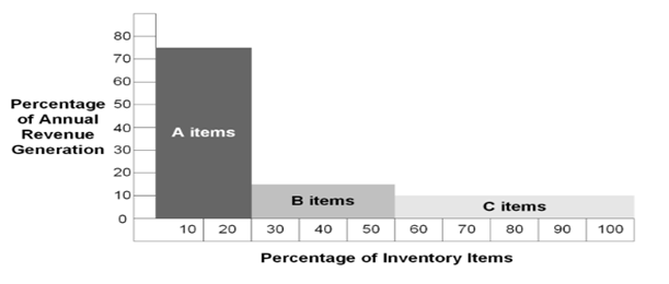
Table 1 — ABC Inventory Classification, Based on Pareto Law

XYZ Inventory Classification

Consumption should be showcased in graphical format on a monthly basis. XYZ classification is based on the consumption pattern where X represents constant demand with rare fluctuations (Figure 1); Y represents seasonal demand or trend with minor fluctuations (Figure 2); and Z represents sporadic demand, completely unstable (Figure 3).

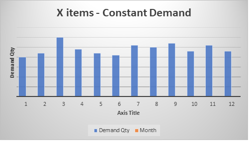
Figure 1 — Constant Demand Items Represented by X

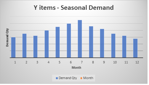
Figure 2 — Seasonal Demand Items Represented by Y

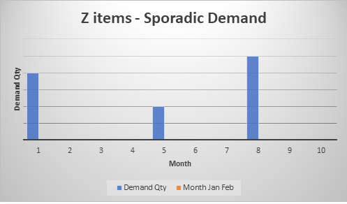
Figure 3 — Sporadic Demand Items Represented by Z

Note: We will cover additional classification categories in the sub-sections.

Item Inventory Management

Item inventory management is used in short-term operational decision making. Management specifies rules to follow for individual inventory items using inventory policy. These rules specify:

• When to order inventory
• How to determine order size
• Relative importance of each inventory item
• Inventory control procedures for individual items

Case Study

A complex manufacturing organization contains four divisions. Each division contains 20 to 30 plants. Across all the plants there are approximately one million materials. Planners within this organization want to classify their materials by consumption value and usage history based on the inventory policy and assign ABC-XYZ classification on material masters to reduce inventory costs and boost up the profits.

Inventory Policy

Group-level materials management defines the inventory policy as shown in Table 2. Category A represents 80% of the consumption value; category B represents 15% of their consumption value; category C represents 5% of the consumption value; category X represents regular demand; category Y represents fluctuating demand; and category Z represents sporadic demand.

• CRM – Customer Relations Management
• VMI – Vendor Managed Inventory
• COV – Coefficient of Variance

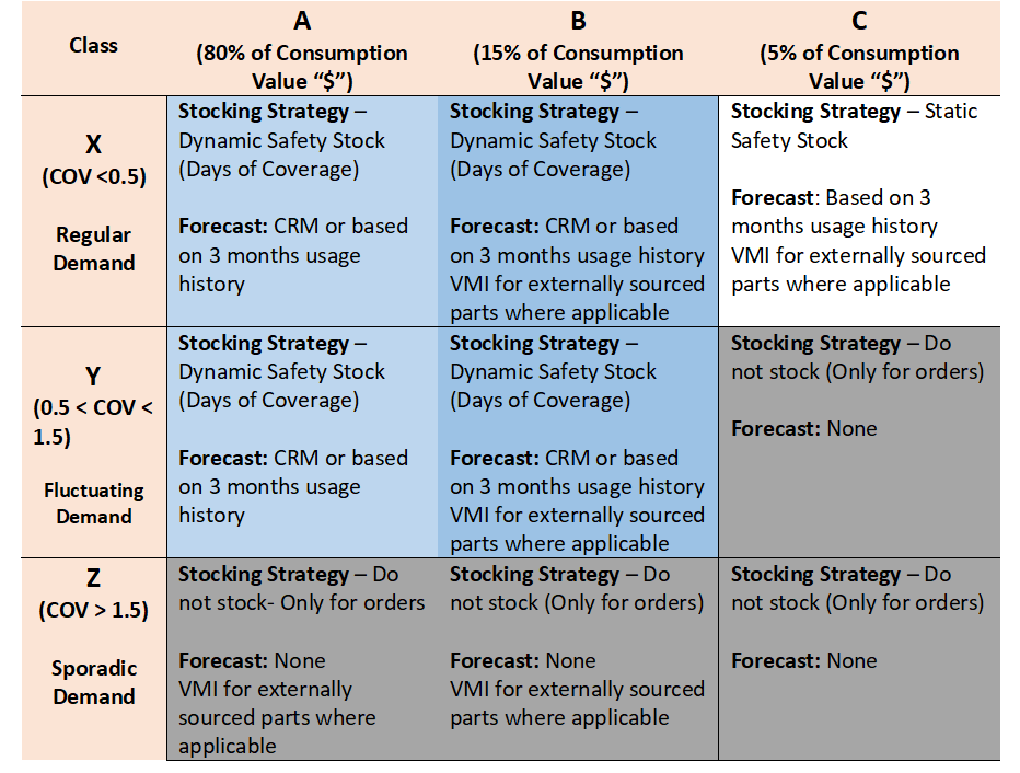
Table 2— Strategic Inventory Policy Guidelines with Forecasting and Stocking Requirements

Materials management teams at the division level should be able to classify the materials on a monthly basis and align SAP material master planning parameters with mass updates to align to inventory policy. This organization cascades this inventory policy to material planners to adhere to the stocking strategy, forecast, and vendor managed inventory policies at the material level, a systematic procedure required to classify materials into ABC/XYZ parameters on a monthly basis.

Organizational Objectives

This organization is into both manufacturing and service with manufacturing plants across the world. Achieving the time to market is one of the primary goals with optimum levels of inventory. The following are the strategic objectives identified by operations management and evaluated on quarterly basis:

• Minimize inventory investment
• Meet targeted level of customer service
• Maximize manufacturing efficiency
• Eliminate manual workarounds to assign safety stocks based on value/consumption-based matrix

Material Document Aggregation (MDA): Purpose and Flow of Information

In this section, you will learn how organizations utilized SAP material document analysis as a first step. In the end-to-end process MDA is used to apply aggregate inventory management rules (primarily concerned with the financial impact of inventories) (Table 2) to determine material specific ABC/XYZ codifications.

The three steps to implement MRP monitor and Inventory Controlling Cockpit are listed below. Each step helps to identify the materials in Table 2 (ABC and XYZ classification). In this article, we are going to discuss the methodology to achieve Step 1 only. Part II of this series will discuss steps 2 and 3.

• Step 1: Execute material document aggregation (MDA)
• Step 2: Import the data into MRP monitor and create a key which can be reviewed as results
• Step 3: SAP Inventory Optimization Cockpit, view graphical and tablet format including deadstock situation

Let’s go over the approach and details on configurations and implementation sequence.

Purpose and Flow of Information

MDA:

• MDA combines consumption data from several material documents into figures that can be analyzed.
• Calculates stock, dead stock, and consumption and stores this data in tables.

 MRP monitor:

• Classifies materials based on business methods, for example, ABC/XYZ analysis (via orders received, consumption, and forecasts).
• The MRP monitor is also an instrument for monitoring master data and key performance metrics.

 Inventory Controlling Cockpit:

• Primarily used to review aggregate inventory level reporting
  • Dashboard
  • Period Comparison
  • Hit list (Top 10 or 25 materials)
• Flexible analysis on ABC/XYZ
• Review ‘Dead Stock’ review at material level.

Figure 4 showcases the purpose and flow of information at a high level, step 1 being MDA.

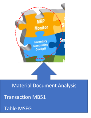
Figure 4 – MDA Outcome is Input to MRP Monitor and Inventory Cockpit

Figure 5 showcases the transactions involved in the implementation approach, bottom up.

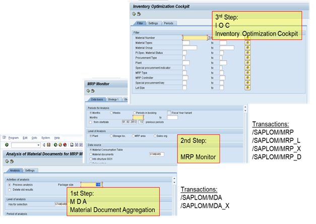
Figure 5 — Implementation Approach Bottom Up

In this three-step process, Figure 6 describes what and how the material document information is scanned and summarized for final reporting.

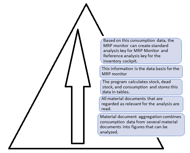
Figure 6 — How Material Document Information is Scanned and Summarized

Relevant Movement Types for Consumption Postings

Analysis of material documents (Transaction: /n/SAPLOM/MDA) is the first step where the business material planning team and IT need to agree upon the settings. This transaction contains two tabs: Analysis and settings.

In the SAP materials management module, when a goods movement is posted, a material document is generated that serves as proof of the movement and as a source of information for any applications that follow.

Material Document and Consumption Overview

When posting a goods movement in the SAP system, a material document is created and can be viewed in MB51 transaction, related accounting docs as per the definition (Figure 7). In this article we focus only on the material documents and its relevance to the objective.

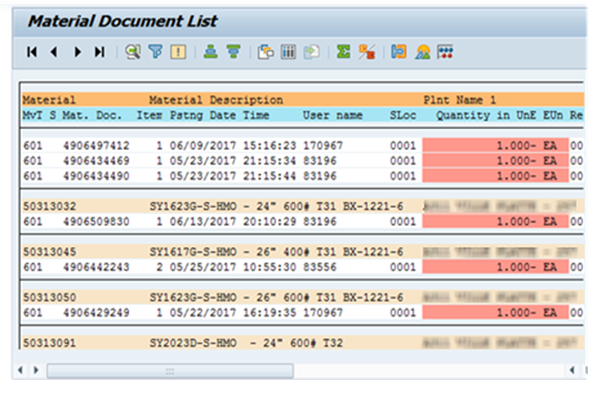
Figure 7 — Transaction MB51 View Material Document List

Figure 8 is an example of 601 moment type configuration highlighting consumption posting field.

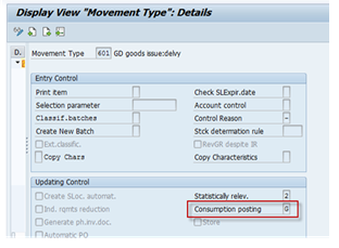
Figure 8 — Consumption Posting Field on Movement Type

Material Document Aggregation: Implementation Approach

In this section you will learn how to set up variants on /n/SAPLOM/MDA and schedule as batch jobs on a monthly basis.

On the selection screen there are two tabs: analysis and settings

Analysis Tab

Figure 9 talks about the selection and the periods (monthly buckets are recommended). Here, you can choose to perform the analysis at plant or storage location level. It is essential that the analysis level you choose here is the same as the one you want to use later in the MRP monitor to review the results.

• Level of analysis: ​You can use this to differentiate between multiple analyses for the same period. STANDARD is always entered here for normal use. Additional document aggregation analysis runs (for special applications or test purposes, for example) can also be stored in the database under different keys, as shown in Figure 9. ​
• Period of analysis: The period of analysis is specified in periods, which enables the date failed to be determined automatically. The end date must always be the current date to ensure that correct starting point is provided, but all the calculations in the document analysis that takes place from the current date backwards (Figure 9).
  • Assign documents to period: You can select creation date, posting date, or document date. I recommend using posting date to execute period assignment. This will provide the realistic situation considering delete times of your products into the right time bucket, as shown in Figure 9.
• Steps for analysis: To perform material document aggregation, all the analysis steps must be executed, but not necessarily in a single aggregation run.

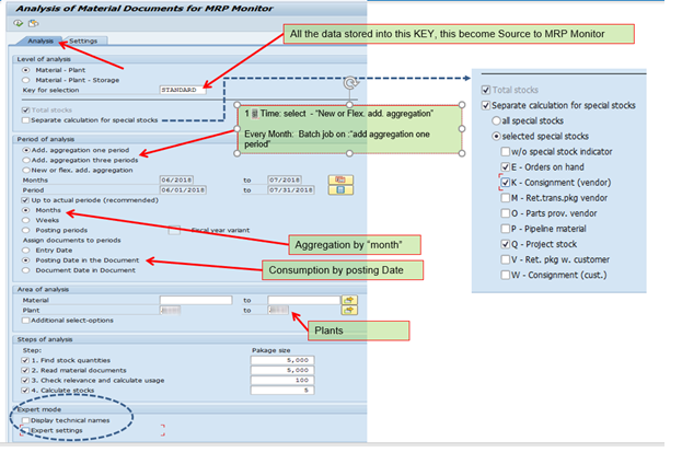
Figure 9 — Material Document Aggregation, Selection Screen

Expert Mode

If a separate analysis is executed for special stocks, you need to decide which additional stocks to include for the respective special stocks. You can specify this on your input screen using corresponding tables and fields, as shown in Figure 10.

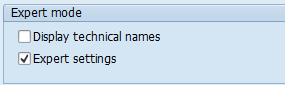
Figure 10 — Expert Mode

Note: If too many fields are selected on the input screen, the system may display incorrect results with excessively high stocks. It is therefore important to carefully check the scenario to be represented in advance.

For expert mode, the following settings must be configured on the Analysis tab page.

Settings Tab

Here the settings define how MTS and MTO inventory movements are captured separately. In standard delivered, there are around 300 plus movement types available (refer to Table T156, Figure 17); however, from an inventory consumption perspective few movement types (around 60 to 70) are relevant for analysis (Figure 9).

Document aggregation always calculates individual stocks based on a starting stock. This is the stock that is available in the system at the time of analysis. The starting stock is therefore an important basis for key figures such as dead stock and inventory turnover.

The starting stock can be read either from the material valuation table (MBEW) or from the info structure statistics: current stock grouping terms (S032), as shown in Figure 11.

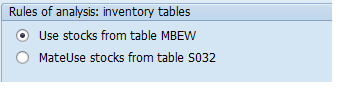
Figure 11 — Analysis of Inventory Tables

Notes:

• In expert mode, the system reads the document from table MBEW by default. Here, in addition to specifying which table is to be used for analysis (MBEW or S032), you can also include valuated sales order stocks (table EBEW), subcontracting stocks (OBEW), and valuated project stocks (QBEW) in the starting stock.
• You first must check whether valuated stocks (tables MBEW, EBEW, QBEW, OBEW) or stock quantities only are relevant for the analysis.
• S032 can only be filled and maintained in your system.

Table Selection for Special Stocks

Organizations should perform either overall calculation or separate calculation for special stocks. In addition, you can analyze all special stocks separately or include selected special stocks only in the aggregation. For later option (special stocks), the individual special stocks can be selected. This means that the analysis by special stocks can be restricted to the relevant time series. Recommended selections are shown in Figures 12, 13, 14 and 15.

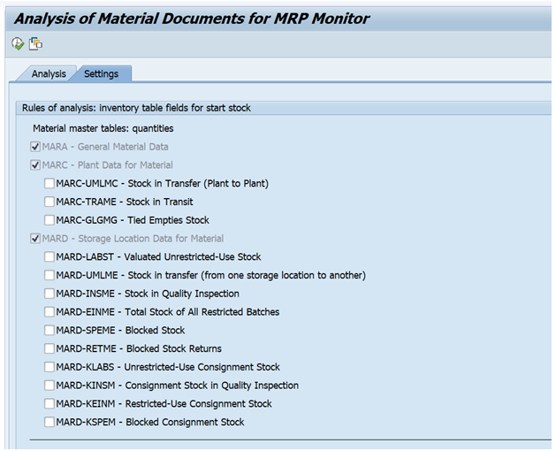
Figure 12 — MDA Analysis Tab, Table for Start Stock

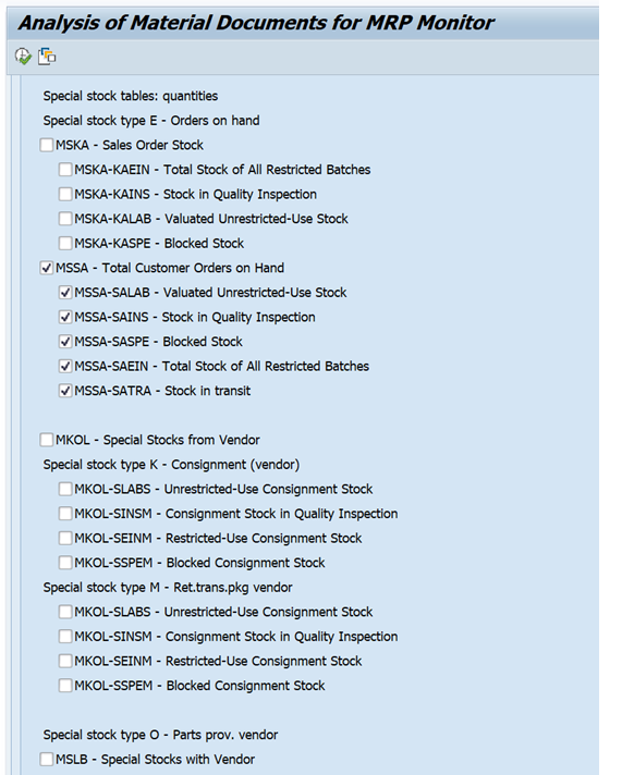
Figure 13 — MDA Analysis Tab, Tables for Special Stock type Orders on Hand

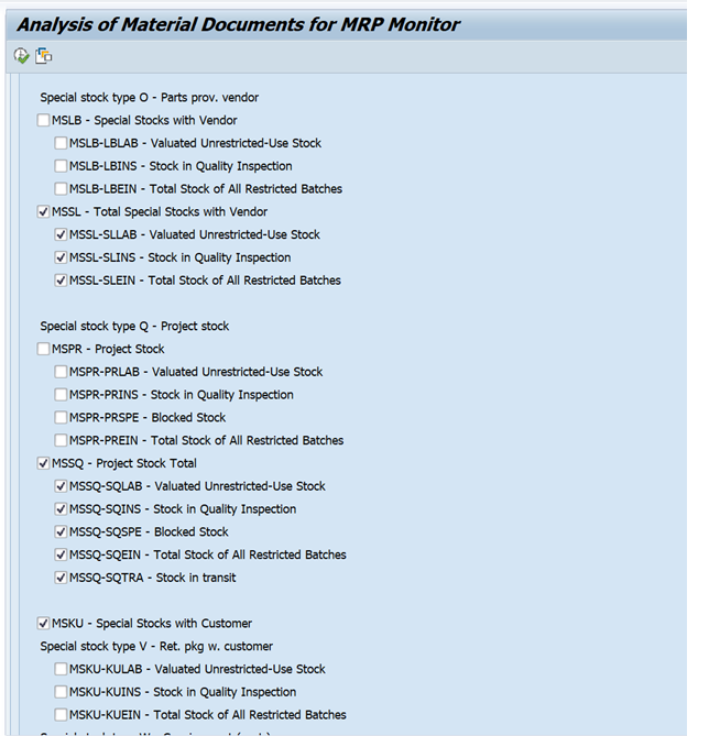
Figure 14 — MDA Analysis Tab, Tables for Special Stock type Vendor, Project and Customer

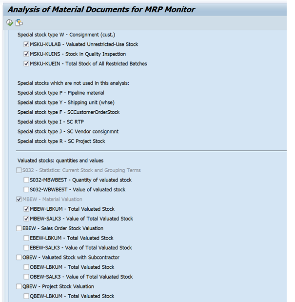
Figure 15 — MDA Analysis Tab, Tables for Special Stock type Consignment & Material Valuation

Analysis Rules for Consumption, Receipts and Stocks Calculation

In this sub section, you should include or exclude the list of movement types and storage locations relevant for consumption, receipts and stock calculations so that this data Is used to generate right aggregate reports In MRP Monitor and Inventory Controlling Cockpit

In the movement types list on the settings tab shown in Figure 16 on both consumption and stock calculation sections, there is an option to exclude few storage locations which are not relevant for calculations. In Figure 16, for example storage location 7000 is excluded because this storage location is used to manage customer property which should not be considered for ABC or XYZ analysis.

Notes:

• Include the movement types used to reverse the consumption as well. For example, movement type 261 is posted when goods issued to production order, so you must include the reversal movement type 262 as well. This will provide correct consumption postings.
• It is recommended to select the check box “Differentiated Evaluation of Movement Types 101 and 102”

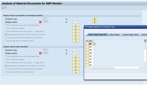
Figure 16 — Analysis of Material Documents for MRP Monitor, Movement Types to Include

Save Variants for Batch Schedule

Once you define the settings mentioned in above sections, save with appropriate name to complete the variant setup of the selected plants. It is possible to have multiple variants for selected plants of the organization as required; include your IT person to optimize the performance.

Create separate variants for each plant if you have few plants in the organization. Or, another way is to create a variant by a profit center where group of plants uses one profit center in large organizations with subdivisions. Each division represents a profit center having multiple plants. This way of maintaining variance is easy and manageable from a scheduling-batch-job perspective on a monthly basis.

How to Find Right Movement Relevant for Consumption Types Using Table and Checking Rules on Movement Types

Organizations’ inventory policies states what type of inventory transactions should be included and excluded in generating reports, so it is crucial to know which SAP movement types are relevant for the analysis of consumption, receipts, and stock calculations. The following sections show how the consultants should analyze using configuration tables and checking rules.

Table Level Analysis

From the SAP configuration table T156, review the list of movement types which are relevant for consumption. The table below defines what each type means (Figure 17).

Note: If consumption posting indicator is G, R, or U, then it is relevant to consumption; if it is blank, then it is not relevant to consumption.

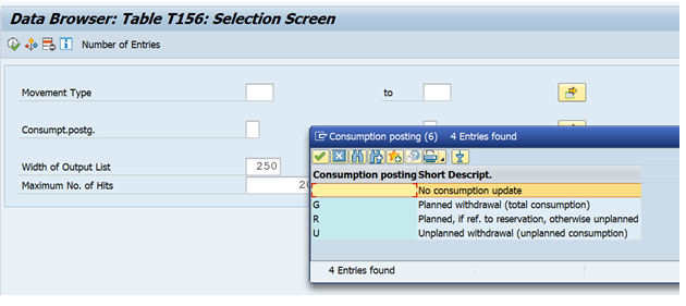
Figure 17 — Table T156 Selection Screen, Consumption Postings

The movement types which have the consumption posting value of G, R, or U should only be considered in the material document analysis setting tab. In standard recipe there are about 300 movement types available but only around 70 are relevant for consumption, as shown in Figure 18.

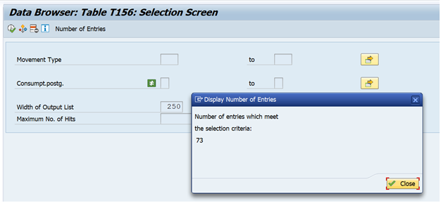
Figure 18 — Table T156 Selection Screen, Movement Types

Checking Rule Analysis

If checking rule “only movement types with consumption flags” rule is activated, then only documents for which the consumption indicator (KZVBU) is set are considered. This is defined in customizing for the movement types. You can see the current settings using transaction OMJJ or in system table T156 (Figure 19).

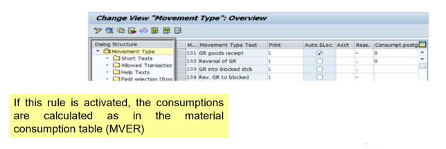
Figure 19 — Overview of Movement Types with Consumption Flags Only

Note: This checking rule applies to stock transfers with a stock transport order. Materials are transferred from one plant to another using movement types 315 (transfer to stock in transit) and 101 (goods receipt). If both documents are included, the receipts are counted twice. The checking rule determines whether the goods movement takes place with reference to the purchase order (KZBEW = B) and whether this is a stock transport order (KZZUG =X) or is posted directly to consumption (KZVBR = V). All these fields can be found in table “Document Segment: Material” (MSEG).

Run material document aggregation as batch jobs

Now that you have set up the variants detailed in table sections, it’s time to run these programs to aggregate the material documents. On the initial run, the material documents from the past two to three years must be aggregated, and on monthly basis, perform material document aggregation for the last period (month)

Initial Run

For the first time, choose “new or flex. add. aggregation” (Figure 20) and define the periods more precisely. It is recommended that you aggregate data for the last three years to ensure meaningful data to determine seasonal materials in the MRP monitor.

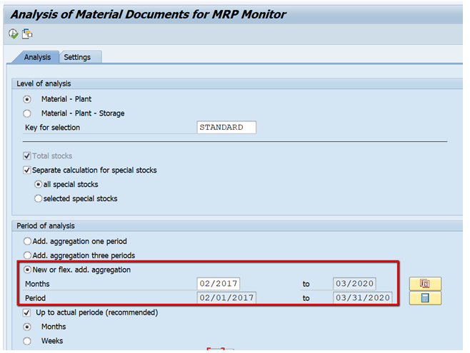
Figure 20 — Analysis of Material Documents for MRP Monitor, Initial Run with Period Range of 3 Years

Periodic Run

Every month you must set up a background job to aggregate data of one period. Choose “Add. aggregation one period” (Figure 21) to select the last fully closed accounting period and schedule these as background job on the third or fourth working day of each month.

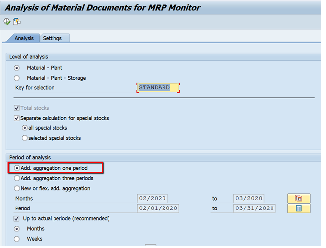
Figure 21 — Analysis of Material Documents for MRP Monitor, Periodic Run

Note: If the “Add. aggregation three periods” is selected, the system aggregates the documents from last three periods, recommended to use only when there are few hundreds of materials (Figure 22).

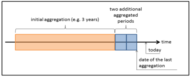
Figure 22 — Material Document Aggregation on Time Scale, Both Initial Run and Periodic Run

Background Logic Used During Material Document Aggregation

The material document analysis shown in Figure 23 executes the following actions for steps of analysis:

1. Find stock quantities

• The current stocks of the materials are read and saved in table STOCK. The wildcard always stands for the prefix /SAPLOM/X_. The table name is therefore /SAPLOM/X_STOCK.
• The starting stocks are calculated and saved in table *START.

2. Read material documents

• All material documents are read and saved in table *BELEG.

3. Check relevance and calculate usage

• Material documents that are relevant for the analysis are filtered out and saved in table *RELEV.
• Date range determination: The dates of the newest and oldest document (first/last usage) are written to table *DATUM.
• Consumption quantities and values are determined per period based on the previously determined documents and the data is stored in table *PERIO.

4. Calculate stocks

• Ongoing stock changes that results from the documents (receipts and issues) are determined and stored in table *BEWEG.
• The daily stocks resulting from the documents are determined and stored in table *DAILY.
• Stocks are determined per period and stored in table *STAND.

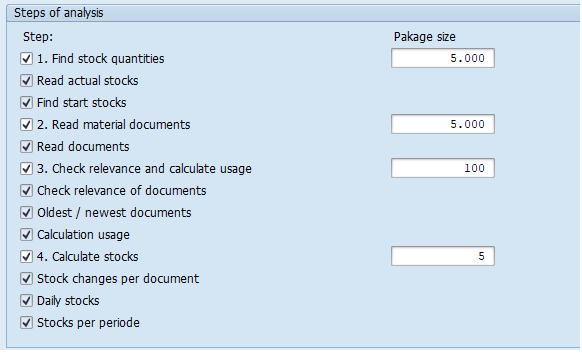
Figure 23 — Steps of Analysis

Tips for Functional and Basis Teams

In this section you will learn tips and tricks on maintenance of the data and how to clean of old results. We’ll also discuss managing the variants on material document analysis and cleanup of old data (typically past 1-2 years) should be performed by IT support team only. The basis team should monitor the table sizes periodically (typically quarterly).

Data Re-organization

If the data stored from previous runs is taking more space than required, you can re-organize a table to gain space. Listed are a few tables. You can refer to the complete list of tables from SE16 with prefix, as shown in Table 3, which showcases sample data on before and after reorganization.

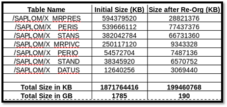
Table 3 — Table Size Before and After Reorganization

• Clean up of old data: IT support team should delete the old reference keys using transaction /n/SAPLOM/MRP_X.
• Batch job run schedule recommended: MDA now runs on the second day of the month to capture all closing activities & the MRPM runs on the third day of the month.
• Deletion of old analyses: You can use the additional program delete for MDA tables to set up aggregations and to free up space in the database that is currently occupied by aggregations that are no longer required; you can access this via transaction /SAPLOM/MDA_X.

Note: Do not delete at table level which may lead into inconsistencies

Performance Optimization by Use of Package Size

Shortage of working memory can be a problem in very large analysis. For this reason, the system can work in package mode. In this mode, only specify the number of materials that are processed at the same time. Table 4 shows recommended settings of packet size in an organization with each variant consisting of approximately 20 to 30 plants with roughly 200K plus material in a single run. Use these recommended values to optimize your batch job schedules.

The mean values represented in Table 4 have emerged from a real-life implementation from large sized- organization having  4 million material across 300 plants.

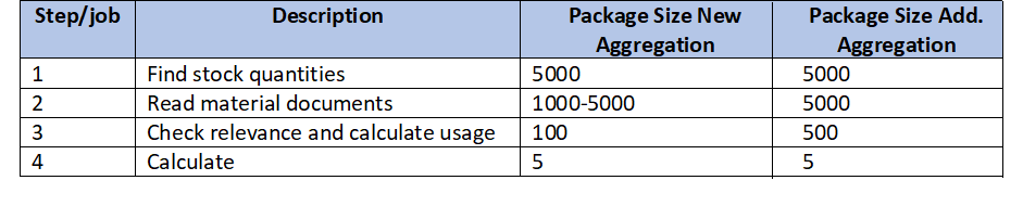
Table 4 — Package Size, Recommended Values

Note: Start with the package sizes mentioned above and gradually determine your own optimum package size. Reach out to SAP support for additional assistance.

The information detailed in this article completes Step 1 of the end-to-end implementation. Refer to Part II of this series for MRP monitor and Inventory Controlling Cockpit.

What Does This Mean for SAPinsiders?

• Inventory policy drives aggregate inventory management. Inventory policy is a way of formalizing the results of strategic inventory decisions so that they can be implemented consistently. Inventory policy codifies both broad and specific inventory management decisions. Factors considered during setting the policy are customer demand, planning horizon, replenishment time, product variety, inventory costs, and customer service requirements. ABC/XYZ classifications should be aligned to the policy and using SAP’s material aggregation tool is one of the best ways to align your SAP system to business objectives.
• Both business and IT must participate on material document aggregation parameters. The material document aggregation is the key step so it is recommended to understand each and every setting and its impact before the variants are set up. Identify the people from the materials management team who have hands-on experience in determining what movement types should be included, identifying specific exclusions, and understanding the aggregation rules. It is very important to understand delete times of the products and identify the initial aggregation.
• Avoid workarounds and utilize SAP tools. In most organizations that analyze materials into value, consumption is very common, and it is a must to make effective decisions. Mostly the data is from tables but extracted into spreadsheets for analysis. For an effective and transparent decision-making process, invest some time into understanding how SAP tools can help to streamline the process so that the planners or inventories specialists productively work and define item level inventory parameters material masters like lot size, safe stock, service level percentage.
• Monitor/measure sizing and performance during implementations. A material document is posted whenever there is a movement of material in the SAP system and the records in the system may end up from thousands to millions on a periodic basis. Therefore, IT experts must analyze the volumes and review the performance settings for effective reporting.